Estimating the fitness of antimicrobial resistance mutations
What you will need:
-BEAST 2.5.0 or greater
-Tracer 1.7.0 or greater
-FigTree
Estimating the fitness of antimicrobial resistance mutations in bdmm
Antimicrobial resistance (AMR) is a growing problem for many microbial pathogens. While it is generally assumed that AMR carries a fitness cost in terms of reduced transmission potential or competitiveness in drug-free environments, the continued spread of AMR strains suggests that resistance may not in fact carry a large fitness cost. A major question surrounding the evolution of AMR is therefore the relative fitness of resistant versus sensitive strains at the host-population level.
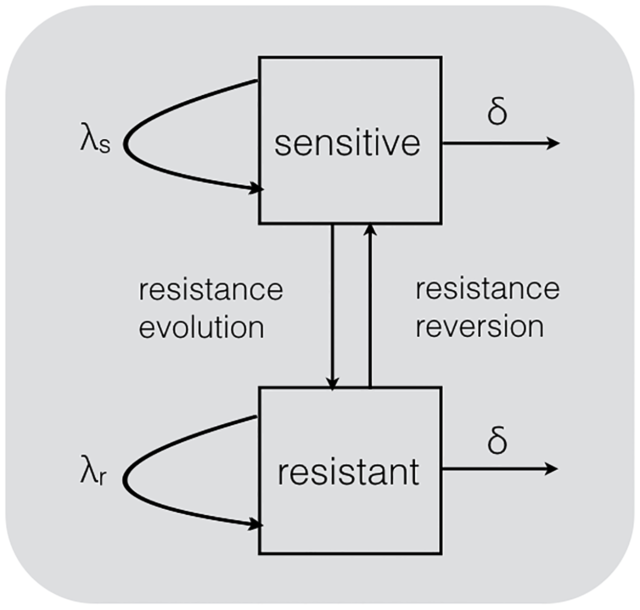
While it is the transmission potential of AMR strains at the population-level that ultimately determines whether or not AMR spreads, measuring pathogen fitness at the population-level is a major challenge. Kühnert et al., (2018) developed a simple but elegant multi-type birth-death (MTBD) model for estimating the transmission fitness of HIV drug resistance mutations from phylogenies. In their model, a pathogen is allowed to transition between resistant and sensitive genotypes, with each genotype having its own transmission rate, \(\lambda_{S}\) or \(\lambda_{R}\). Fitting the MTBD to HIV phylogenies thereby allowed the authors to estimate the relative transmission fitness of different resistance mutations.
In this tutorial, we will use bdmm, a BEAST2 package for phylodynamic inference using multi-type birth-death models (Kühnert et al., 2016), to estimate the fitness of resistant and sensitive genotypes from phylogenies.
The simulated data
We will analyze a simulated data set containing both sensitive and resistant genotypes of a generic pathogen. This will allow us to test whether we can estimate the true fitness of each genotype known from the simulations.
I first simulated a pathogen phylogeny under a simple two-strain birth-death model. I then generated mock sequence data by simulating sequence evolution along each branch of the phylogeny using pyvolve. The sequence data was assumed to evolve neutrally and independently of the resistance genotype. The simulated phylogeny and script I used to generate the sequence data are available here if you’re interested.
You can download the simulated sequence data as a FASTA file using the link below:
Installing bdmm
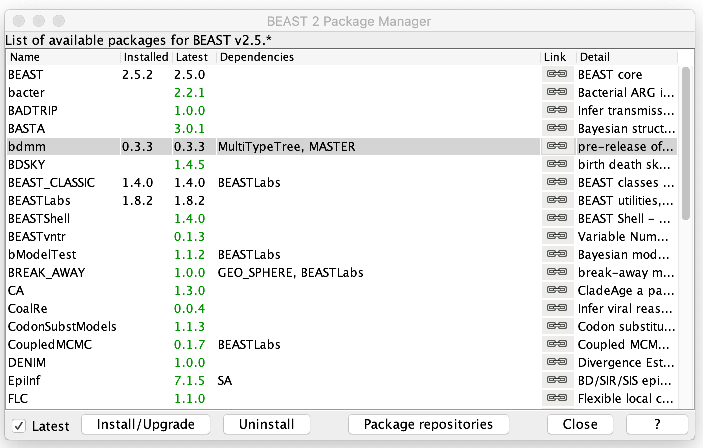
Open BEAUTi and select File → Manage packages. Select bdmm and then hit Install/Upgrade. The bdmm package also requires MASTER and MultiTypeTree as dependencies, but these should be automatically installed with bdmm. Make sure to restart BEAUTi once bdmm has been installed so the changes take effect.
Setting up tip dates and locations
Once you reopen BEAUTi, go to File → Template and then select MultiTypeBirthDeath. This will let BEAUTi know that you want to use this template to generate the XML input for BEAST.
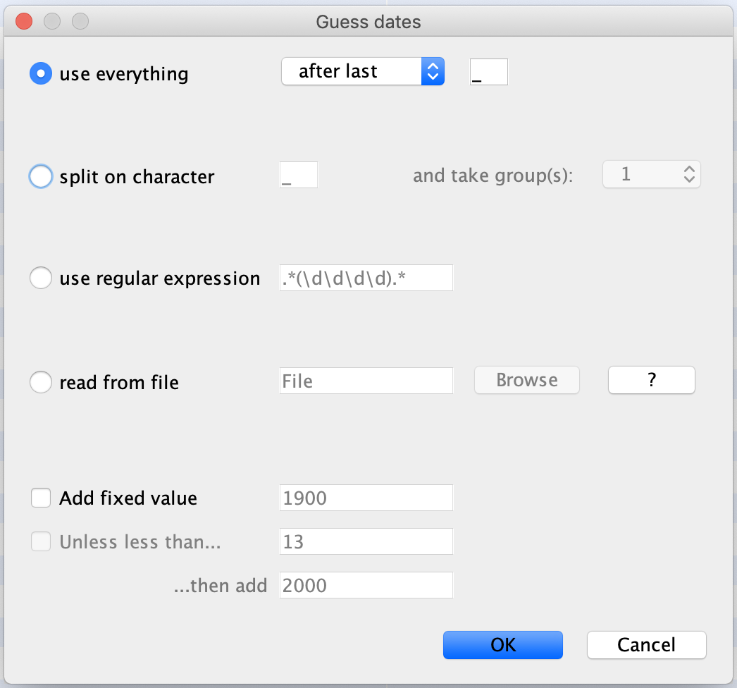
Load in the AMR-seqsim.fasta alignment file you downloaded through File → Add Alignment. Under Tip Dates select ‘Use tip dates’ and then hit Auto-configure. The sampling dates are encoded in the sample names after the last underscore, so select ‘use everything’, ‘after last’, ‘_’. Then hit OK.
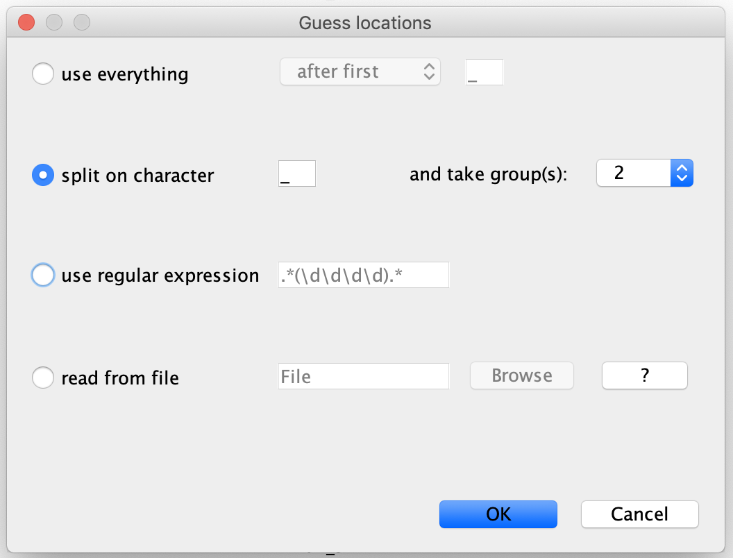
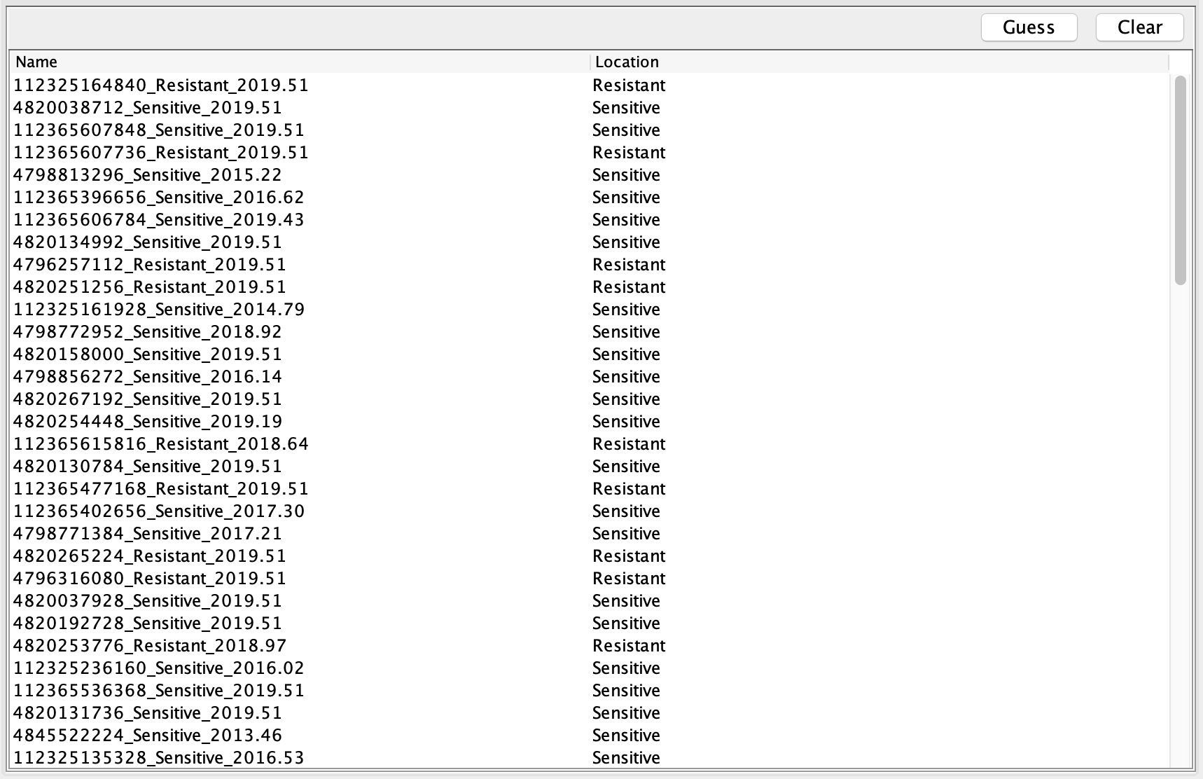
Next go to the Tip Locations panel and select Guess. In the Guess locations box, select ‘split on character’, and choose take group(s) ‘2’.
The genotype of each sample should then be displayed under ‘Location’ as either sensitive or resistant:
Setting up the Site and Clock Model
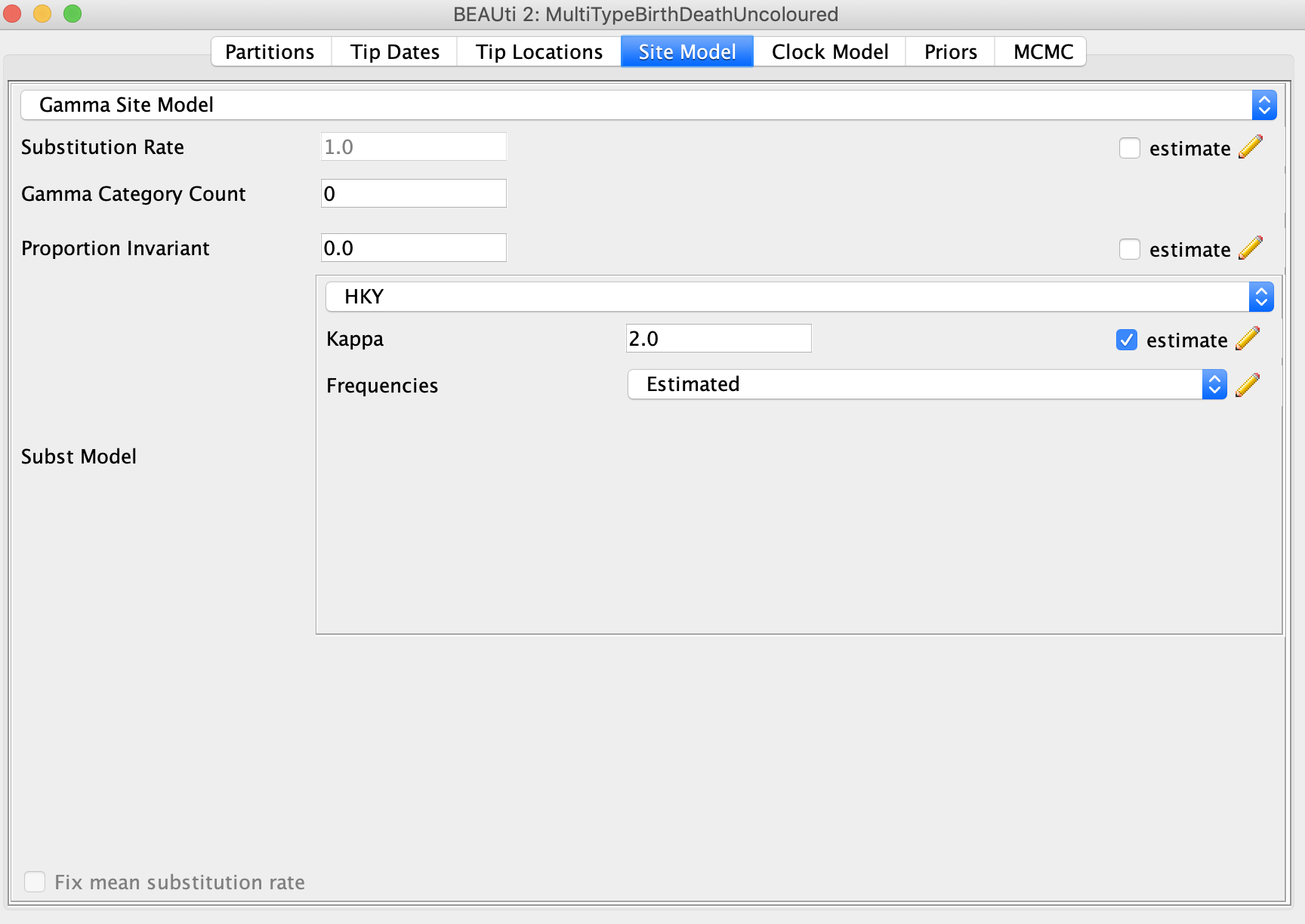
Select the Site Model panel. I simulated the sequence data under a HKY model with no rate heterogeneity across sites, so in this case we know the exact substitution model. Because there is no rate heterogeneity we can set Gamma Category Count to zero. For the substitution model, select HKY. It might be interesting to see if we can correctly estimate the correct Kappa transition-transversion ratio I used to simulate the sequences, so select estimate next to Kappa. The true value is 2.75.
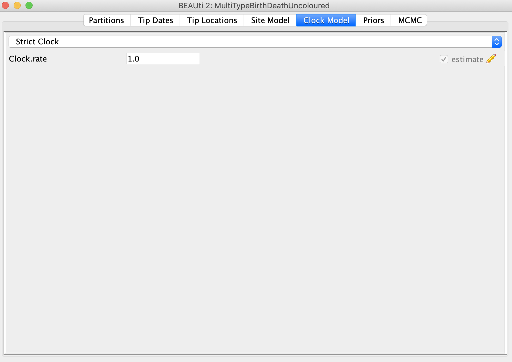
Under the Clock Model panel, select Strict Clock and check the estimate box next to Clock.rate. The true value I used in the simulations is 0.005 substitutions per site per year. You may want to initialize the Clock.rate closer to this value so that the BEAST MCMC converges quicker.
Setting up the bdmm tree model
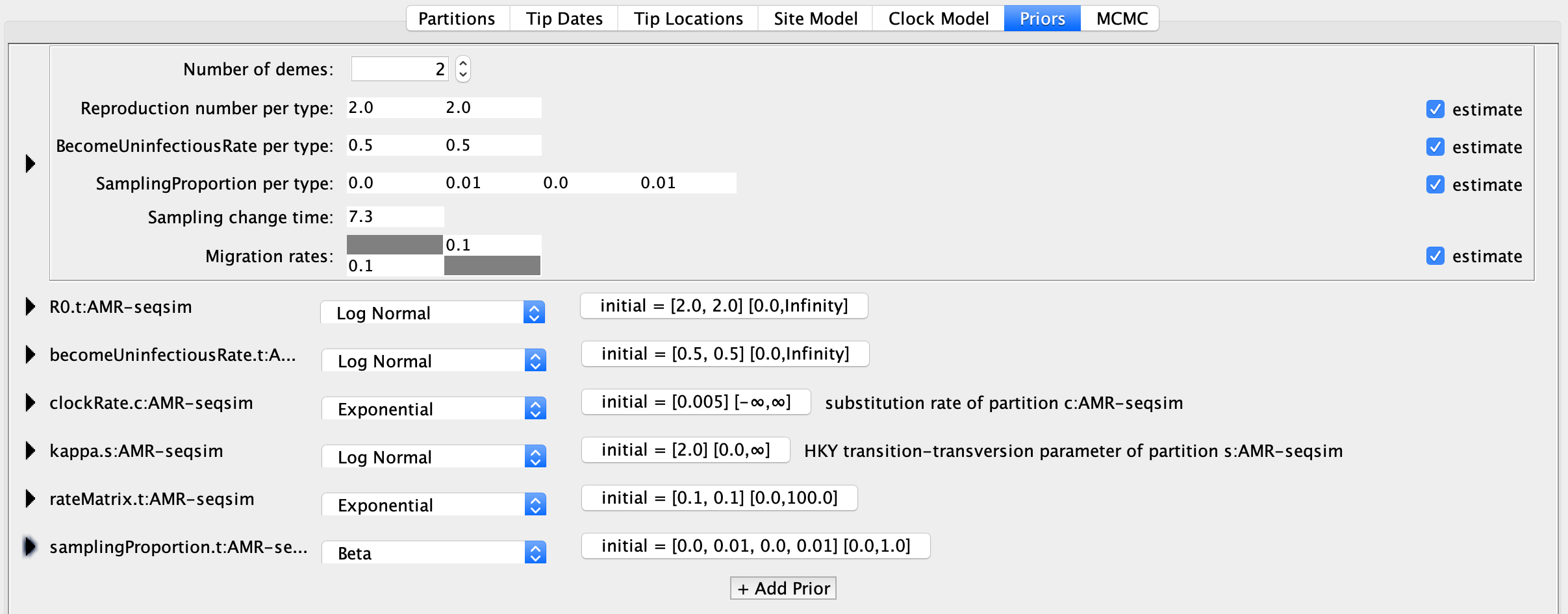
That should have all seemed rather familiar by now. Next, we will set up the multi-type birth-death model itself. Go to the Priors panel and you should see the MTBD model parameters at top. Note that the BEAUTi interface assumes that the types in the model are different locations, and refers to these as demes. This isn’t a problem, we just need to think of the demes as the different genotypes in our model. Under Number of demes make sure there are two demes.
In our analysis, we are mainly interested in estimating the Reproduction number per type, which is the \(R_{0}\) value for each genotype. You can keep the initial values at 2.
Remember that under a birth-death model we cannot jointly estimate the transmission rate, death rate and sampling proportion together. We can only estimate two of these parameters. Because we do not know the true sampling proportion and are interested in estimating the transmission rates in terms of \(R_{0}\), we will provide the death rate. In BEAUTi, the death rate is called the BecomeUninfectiousRate (catchy, huh?). The reciprocal of this value gives the average duration of infection. In my simulations, hosts stayed infected for an average of two years, regardless of the pathogen genotype, so the true BecomeUninfectiousRate is 0.5. We could fix this parameter at its true value, but we will adopt a more refined Bayesian approach and specify an informative prior on the BecomeUninfectiousRate below. For now, we can change the initial values for both types to 0.5.
Let’s skip ahead to the Sampling change time parameter, which allows the sampling proportion to change at a given point in time. The default configuration allows the sampling proportion to change at one point in time because it is recommended by the developers of bdmm that the sampling fraction be set to zero before the time of the first sample. This turns out to be a very sensible thing to do because we know ipso facto that the sampling proportion must be zero before the first sample, and there may be a very long period of time separating the root from the first sampling event. Thus, our estimates of the sampling proportion would likely be biased downwards if we did not account for no sampling before the first sampling event.
The time of the earliest sample is 7.29999 years in the past, which can be verified by looking at the tip heights under the Tip Dates panel. bdmm expects times to be specified in time since the present, so will set the Sampling change time to 7.3. Rounding up here ensures that this change point occurs earlier (further in the past) than the first sampling event.
Note: Time-varying parameters
In our analysis we let the sampling proportion change through time. But actually any of the MTBD parameters can be made to vary over time in a piecewise constant manner. Unfortunately, this cannot be done in BEAUTi and needs to be set up manually in the XML file. So we will not consider other time-varying parameters for now.
Now we will return to the actual SamplingProportion per type parameter. There are four values listed here, the first two values correspond to the two sampling time intervals for the first type, and the third and fourth values correspond to the two sampling time intervals for the second type. Make sure the first sampling interval for each type (i.e. the first and third values) is set to zero. The default value of 0.01 is fine for the sampling proportion after the Sampling change time.
The Migration rates correspond to the mutation rates between resistant and sensitive genotypes. We can leave these at their default values. The Priors panel should now look like this:
Setting up the prior distributions
Now we need to specify a prior distribution on all model parameters. You can click the right facing arrow next to each variable in the Priors panel to see a drop down menu in which you can specify the prior values.
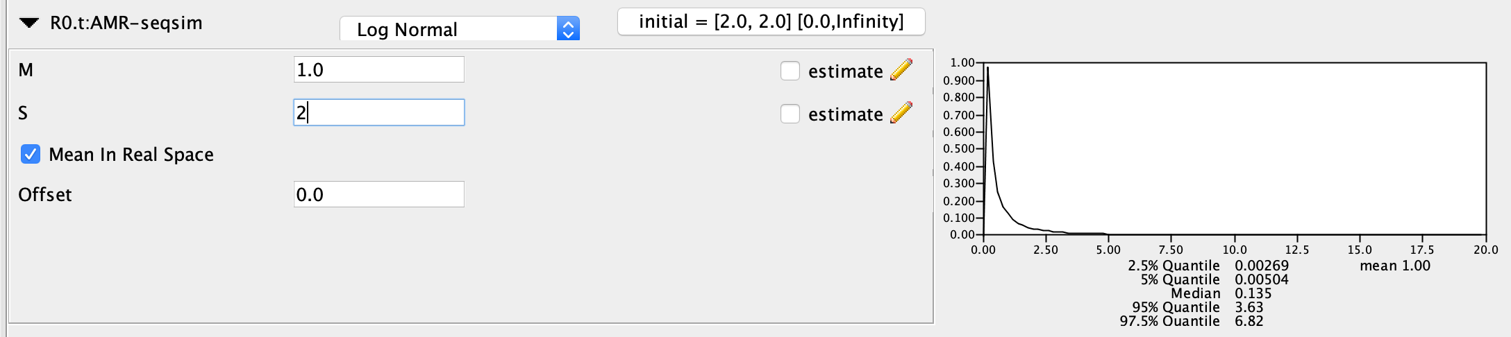
For \(R_{0}\), I recommend a fairly uninformative prior since we truly do not know the \(R_{0}\) for each genotype, and do not want our prior to strongly influence our estimates. I set a Log Normal prior with mean (M) = 1.0 and a standard deviation (S) = 2.0. Make sure ‘Mean in Real Space’ is checked so that we are not specifying the mean on a log scale. This places most of the prior probability between 0 and 3, which is reasonable because only extremely infectious pathogens will have a \(R_{0}\) above 3.
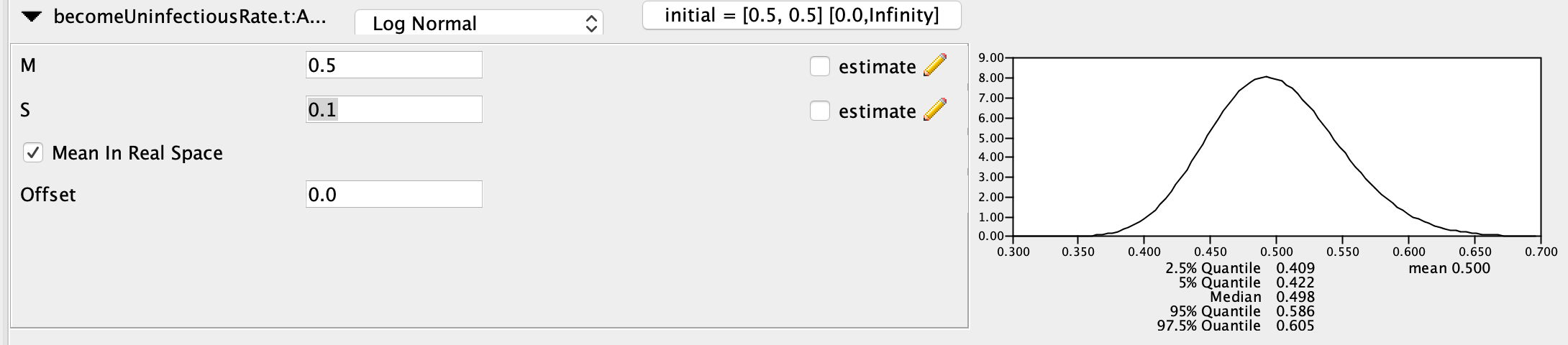
On the other hand, we will use a highly informative prior for the becomeUninfectiousRate, otherwise we will not be able to infer \(R_{0}\) and the sampling proportions. The true rate is 0.5 so I chose a Log Normal prior with mean (M) = 0.5 (again in real space) and S = 0.1, which places most of the prior probability between values of 0.4 and 0.6.
For the clockRate prior, I used an Exponential prior, with a mean of 0.01. An Exponential prior is a reasonable choice whenever parameter values need to be positive (like for rates), but we have reason to believe that higher parameter values become increasingly less probable. For kappa I kept the default Log Normal prior.
The rateMatrix priors are for the mutation rates in the MTBD model. I used an Exponential prior with the default mean value of one.
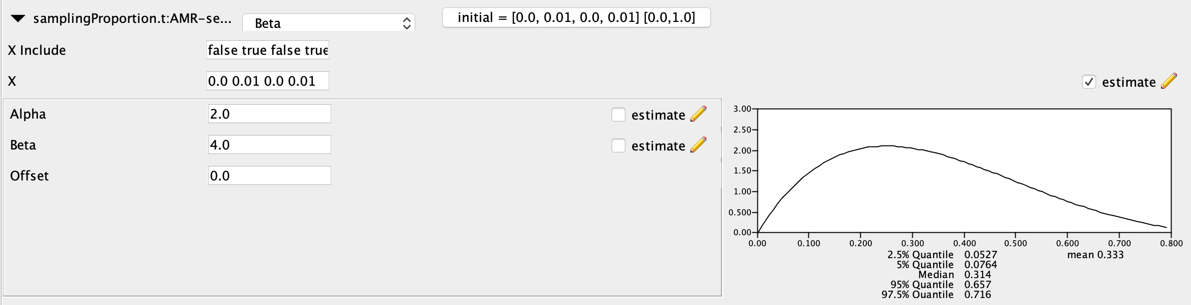
Finally, for the prior on the samplingProportions I used a Beta prior. The Beta distribution is a natural choice for parameters like frequencies or proportions that are constrained to values between zero and one. The alpha parameter of the Beta distribution controls the overall shape of the distribution, including how flat or peaked it is. The beta parameter controls the skew of the distribution towards 0 or 1. I set alpha = 2.0 and beta = 4.0 to indicate my prior belief that samplingProportions below 0.5 are more probable than values above 0.5, with the distribution centered around 0.25. We can leave the ‘X include’ values as [false true false true]. This just tells BEAST that we don’t want to estimate the samplingProportions in the time interval before the first sampling event.
Running the analysis in BEAST
In the MCMC panel, set the Chain Length to 2,500,000 iterations. Then navigate to File → Save to generate a XML input file that you can then run in BEAST.
Posterior analysis in Tracer
The MCMC run took approximately 25 minutes to run on my laptop, so hopefully your run will finish before the end of class too! If its taking too long, you may want to download my pre-cooked .log and .trees files.
Open the .log file in Tracer so we can examine our posterior estimates of the MTBD and substitution model parameters.
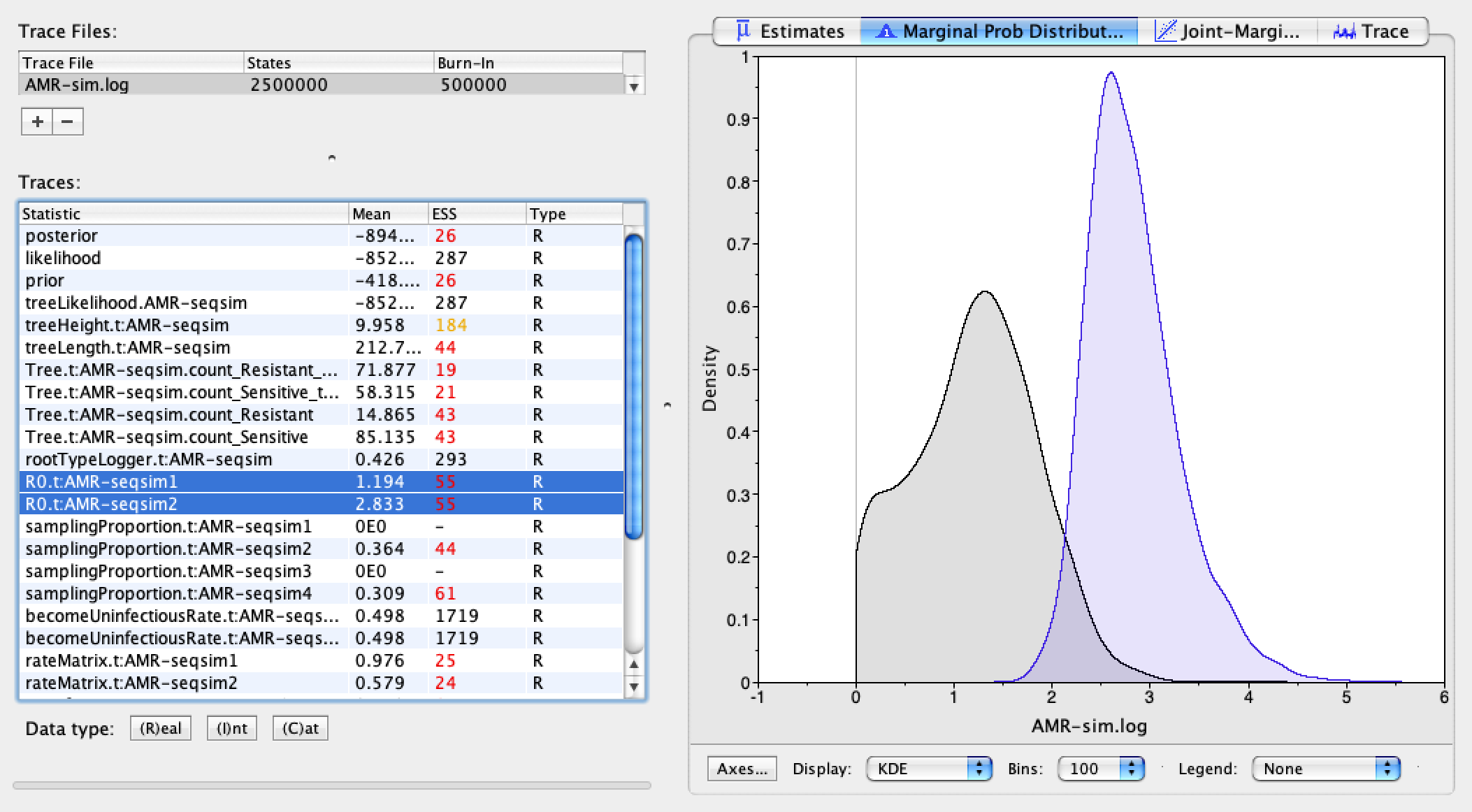
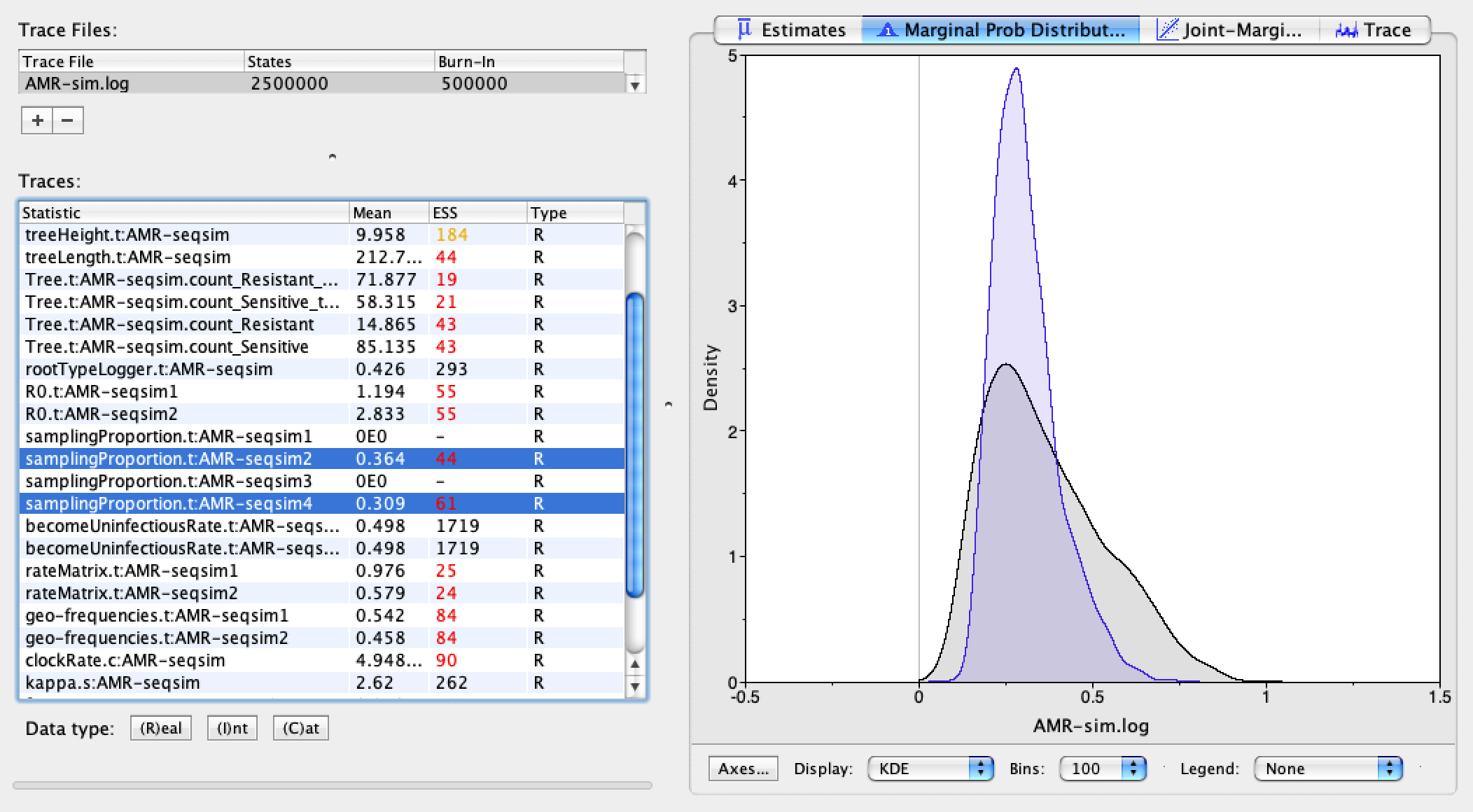
First let’s look at the estimated \(R_{0}\) values for the sensitive and resistant genotypes. Select the two \(R_{0}\) parameters in the window on the left and then look at the Marginal Prob Distribution. The first value is for the resistant genotype and the second is for the sensitive genotype. We can see that the \(R_{0}\) for the sensitive genotype is more than twice that of the resistant genotype. In the simulations, the true ratio of \(\frac{\lambda_{S}}{\lambda_{R}}\) was 2.0, so the estimated ratio of \(R_{0}\) values is not far off from the truth.
The posterior estimates for the becomeUninfectiousRates are centered around 0.5 and remained within the 0.4 to 0.6 interval, so were clearly constrained by our prior, as expected.
The median posterior estimates for the samplingProportions are 0.36 and 0.31 for the resistant and sensitive genotypes, respectively. The true sampling proportion was 0.25 for both genotypes, so again the estimates are not far off.
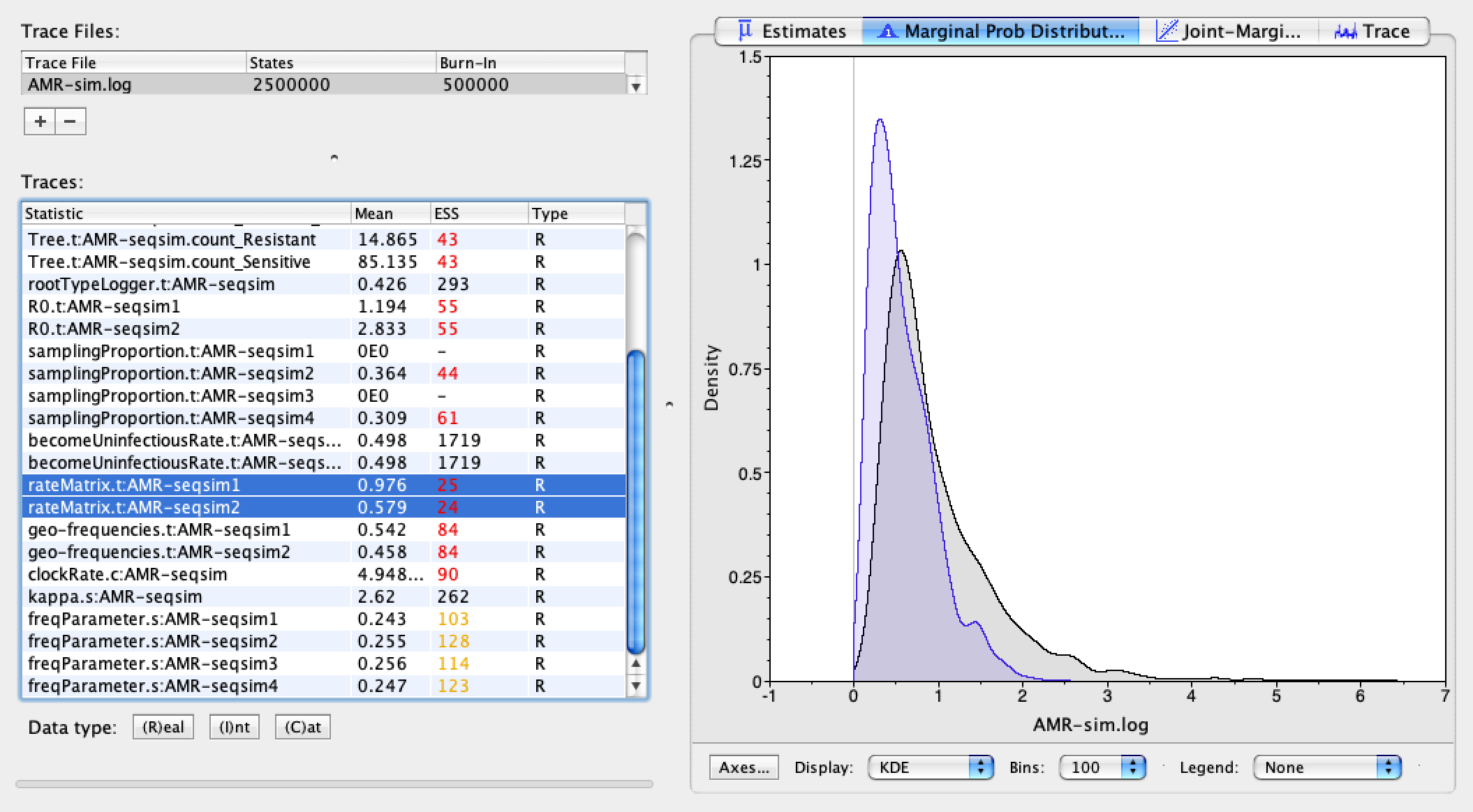
Next we can examine the rateMatrix estimates for the mutation rates between resistant and sensitive genotypes. The true mutation rates were 0.2 in both directions, so we overestimated these rates, but there is also substantial uncertainty surrounding our estimates.
Finally, we can examine our estimates of the substitution model parameters, kappa and the molecular clockRate. The true values I used to simulate the sequence data were kappa = 2.75 with a clockRate of 0.005, so it appears we very accurately and precisely estimated these parameters.
Visualizing ancestral type trees
We can also look at the ancestral types bdmm reconstructed for the nodes and branches in the inferred phylogenetic tree.
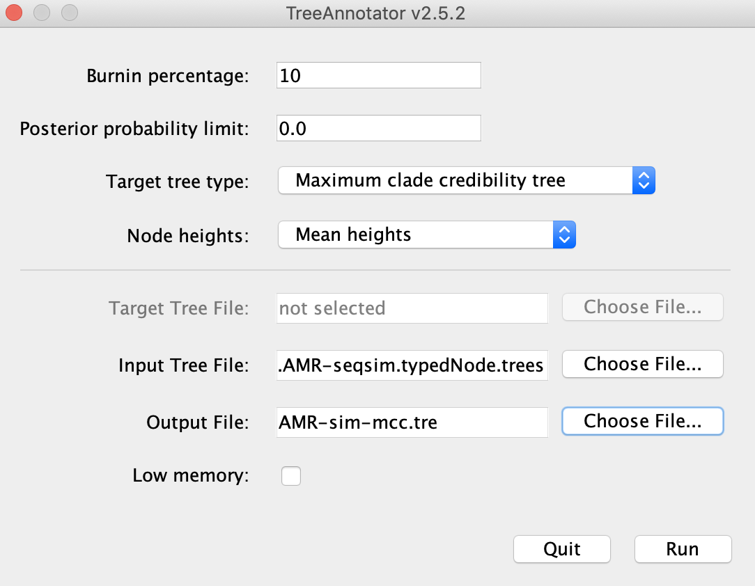
Open TreeAnnotator and for Burnin percentage choose 10%, for Target tree type select Maximum clade credibility tree and for Node Heights select Mean heights. For the Input Tree File select the .trees file with typedNodes in the name. These are the trees BEAST sampled with ancestral types mapped onto the tree nodes. Choose an Output File name and then hit Run.
Open the resulting MCC tree in FigTree. Go to Appearance → Colour by → type to color the tree by the reconstructed ancestral genotypes. To get posterior probabilities on the ancestral types, go to Node Labels → Display → type.prob. This will display the posterior probability of each node having the sensitive genotype.
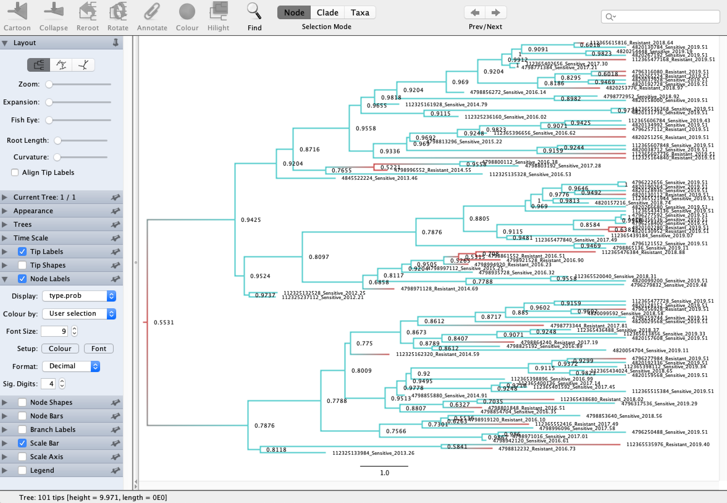
We can see that most of the transmission/branching events in the tree involved sensitive genotypes and that the resistant genotypes are mainly restricted to single tips or cherries in the tree. Its therefore not too surprising that we estimated the sensitive genotype to have much higher fitness than the resistant genotype.
References and further information
This tutorial was partially based on an earlier BEAST2 bdmm tutorial by Denise Kühnert and Jūlija Pečerska.