Structured coalescent inference with MASCOT
What you will need:
-BEAST 2.5.0 or greater
-Tracer 1.7.0 or greater
-FigTree
Structured coalescent methods
Most host populations are structured into different subpopulations, either by geographic isolation or other divisions. Extending coalescent models to include population structure allows us to account for population structure when estimating other demographic parameters and to reconstruct the movement of individuals between populations. Early structured coalescent methods such as MIGRATE (Beerli and Felsenstein, 2001) allowed population sizes and migration rates between multiple populations to be estimated from phylogenies, but required migration histories to be estimated along with these parameters using MCMC. The need to sample migration histories caused these early structured coalescent methods to be computationally inefficient when applied to large trees with samples from many populations. Newer approximations to the structured coalescent try to ease this computational burden by integrating (i.e. summing) over all possible migration histories when computing the likelihood of the phylogeny (Volz, 2012; De Maio et al., 2015; Müller et al., 2017). In this tutorial we will explore MASCOT (Marginal Approximation of the Structured COalescent), which uses an improved approximation to the structured coalescent to estimate model parameters and reconstruct ancestral states (Müller et al., 2018).
Reconstructing the early spread of Ebola virus in Sierra Leone
In 2013-16, a large Ebola virus (EBOV) epidemic infected over 26,000 people in western Africa. The epidemic spread quickly between geographically isolated locations (Dudas et al., 2017). Here, we will use MASCOT to reanalyze the viral genomic data of Dudas et al. (2017) in order to reconstruct the early spread of Ebola through Sierra Leone. We will also explore how well different spatial covariates predict the spread of Ebola using Generalized Linear Models (GLMs).
The EBOV Data
The original dataset of Dudas et al. (2017) contained 1610 full viral genomes sampled from Sierra Leone and neighboring countries. To speed up our analysis, we will examine a subset of this data containing 77 sequences for the non-coding portion of the EBOV genome. An aligned FASTA file containing these sequences can be downloaded using the link below:
To predict migration rates, we will use great circle distances between districts in Sierra Leone and a binary predictor that encodes whether or not two districts share a common border. CSV files containing these spatial covariates can be downloaded using the links below:
We will also use human population densities and weekly case reports from each district as a time-varying predictor of effective population size changes through time:
Installing MASCOT
To install MASCOT, open BEAUTi and navigate to File → Manage Packages. Currently, the MASCOT-GLM models have only been implemented in a pre-release of MASCOT v 2.0. To install this pre-release, click on Package repositories and then Add repository. Copy and past the following URL into the Add repository URL text prompt: https://raw.githubusercontent.com/nicfel/Mascot/master/package.xml.
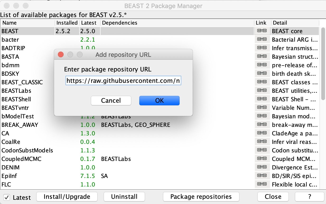
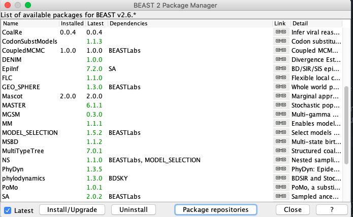
Click OK and the new URL should now be displayed under the Package repository URLs. Click Done and return to the main package manager window where you can now select MASCOT and press Install/Upgrade. The installed version of MASCOT should now appear as 2.0.0.
Important: Remember to restart BEAUTi after installing MASCOT otherwise the changes will not take effect.
Loading the EBOV sequences and sampling times
The sequence alignment is in the ebov_noncoding.fasta you already downloaded. From the Partitions panel in BEAUTi select File → Import Alignment and choose this FASTA file. Make sure that you specify that this is a nucleotide alignment and not an amino acid alignment.
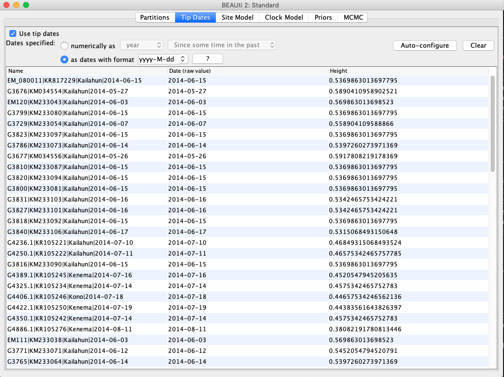
Move to the Tip Dates panel and then select the Use tip dates checkbox. The sampling times are already encoded in the sample names so we just need to parse them. First, set the as dates with format to yyyy-M-dd. Then click the Auto-configure button. The sampling times appear following the third vertical bar “|” in the sample names. To parse these times, select split on character, enter “|” (without the quotes) in the text box immediately to the right, and then select “4” from the drop-down box to the right. The sampling times should now appear in the Tip Dates panel.
Setting up the Site and Clock Model
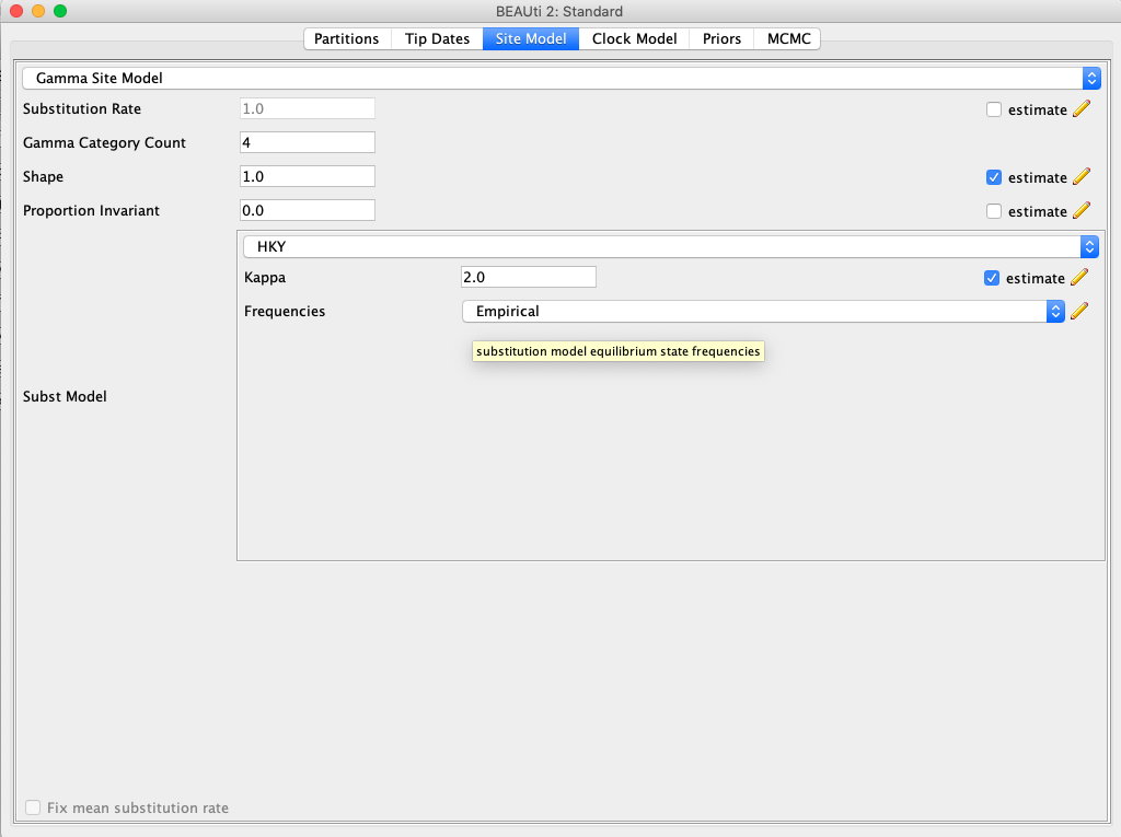
Click the Site Model tab at the top of the window to specify a substitution model. We will use the HKY model, which is simpler than the GTR model but still accounts for differences in transversion versus transition rates. Additionally, we will allow for rate heterogeneity among sites by changing the Gamma Category Count to ‘4’. Make sure that estimate is checked next to the shape parameter. To reduce the number of estimated parameters, we can set Frequencies to be Empirical.
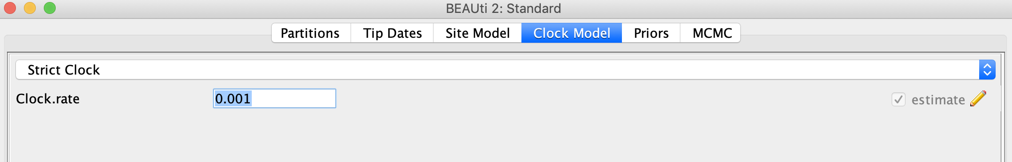
Next click the Clock Model tab to set up the molecular clock model. Our sequence samples are collected serially over time, so we can estimate the clock rate based on the sampling times. To help BEAST converge faster, we will start with a reasonable clock rate of 0.001 substitutions per site. Leave the Strict Clock option selected in the menu at top and type this rate into the Clock.rate box.
Setting up the MASCOT-GLM Model
Next, go to the Priors panel. At the top, choose Mascot from the drop down menu where the different tree priors can be specified. Click the right facing arrow to the left of this menu to expand the options under the MASCOT model. In the second drop down menu immediately below select GLM. The panel should now look like this:
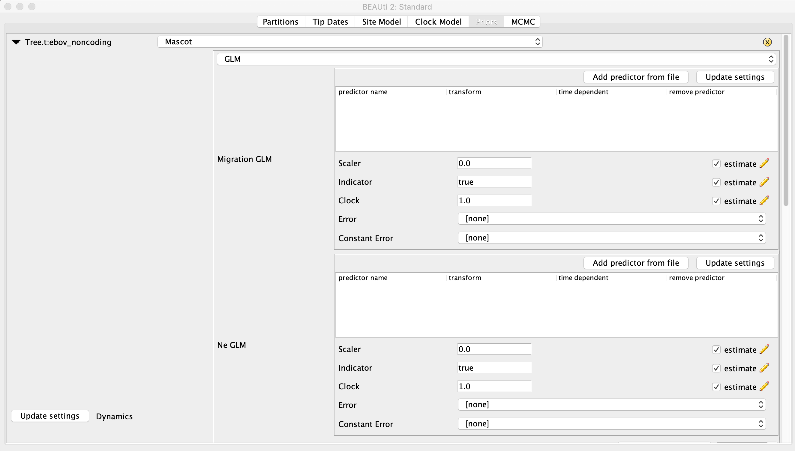
To get orientated, you should see two boxed-off menus for setting the Migration GLM predictors and the Ne GLM predictors. Below these menus there will be a table with the name and location of each sample.
WARNING: The BEAUTi graphical interface for the MASCOT-GLM models is still under active development and can be quite finicky. Make sure you follow the next few steps very carefully or errors will likely occur.
Parsing the sampling locations
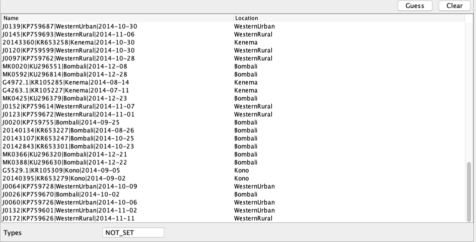
We now need to set the sampling locations. As with the sampling times, the sampling locations can be parsed from the sample names. Scroll down to the table with the name and location of each sample. After clicking the Guess button, you can split the sequence on the vertical bar “|” again by selecting “split on character” and entering “|” in the box. The locations are in the third group, so choose “3” from the drop-down menu. After clicking the OK button, the window should look like this:
Setting up the time-varying predictors of Ne
We have two types of predictor variables: constant predictor variables like the population densities and time-varying variables that we will use to predict changes in effective population sizes through time. If we look at the case report data in the Ne_cases.csv file, you will see that there are weekly case reports for each location. We need to associate these case reports with specific dates and let the model know when to switch between entries.
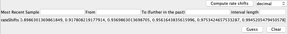
Here, the case data is specified on a weekly basis and we therefore have to specify when to change between weekly entries. We do this be setting the rate shifts. First, in the text box next to Compute Rate Shifts, change the format in which the dates will be specified from decimal to yyyy-MM-dd. The most recent sample was sampled on 2014-12-28. This can be checked by going back to the Tip Dates panel and finding the sample with height 0. For Most Recent Sample enter “2014-12-28”.
The next thing we need to define is when the most recent entry of the predictor variables is from. The most recent entry defines the weekly case count in the week of 2015-11-16, which will be our From value. The last entry of the case data is from 2013-12-30, which will be our To value. The Interval Length defines how much time there is between different entries of the predictor. Since we have weekly cases, this is 7 days. We input this is in the same date format as all the other values, i.e. 0-0-7. To summarize, the entries should look like this:
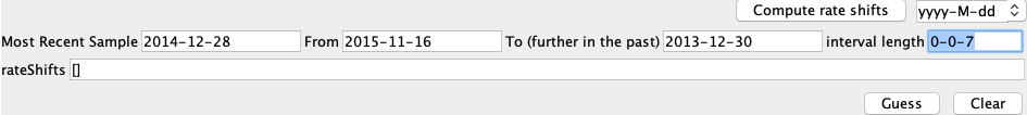
Next, press Compute rate shifts, which will convert the date information into decimal values. Becasue the most recent sample is further in the past than the most recent predictor entry, the first entries of rate shift will be negative. The rateShifts values should now be populated:
After all this is setup, make sure to hit Update Settings on the left. This is absolutely crucial for adding predictors. BEAUTi will automatically make sure that the dimensions of the predictor variables are correct based on how many different locations and rate intervals we have set.
Adding the predictor data
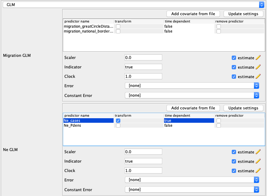
First we will add the migration rate predictors. To load the predictors, in the Migration GLM box press Add predictor from file and select the file migration_greatCircleDistances.csv. This predictor denotes the log-standardized distances between the population centers of each location. Next, add the predictors in the migration_national_border_shared.csv file. This predictor denotes if two locations are located next to each other.
So what are we actually doing here? In essence, we’re setting up a (multiple) linear regression model where the log-transformed great circle distance \(D_{ij}\) and the shared boarder data \(\epsilon_{ij}\) predict the migration rate \(m_{ij}\) between each location \(i\) and \(j\). So we have a model that looks like this:
\[m_{ij} = \beta_{0} D_{ij} + \beta_{1} \epsilon_{ij},\]where we will estimate the regression coefficients \(\beta_{0}\) and \(\beta_{1}\) that determine the effect size of each predictor variable using BEAST.
Now we will add the effective population size predictors. In the Ne GLM box, add the predictors in the Ne_cases.csv and Ne_Pdens.csv files. The predictor Ne_cases denotes the number of weekly case reports. The timepoint 0 is always the most recent time interval and earlier time intervals are denoted as 1,2,3….. These cases are not yet log-standardized and so we have to click the transform button next to the predictor name. After doing so, click the Update Settings button again.
Note: Because log(0) is negative infinity, 0 values in the case reports haven been replaced with a value of 0.001 in weeks where there are no reported cases.
The GLM setup should now look like this:
Specifying the other priors
Now, we need to set priors on the various other parameters in the model. The NeClockGLM and migrationClockGLM variables are priors on the overall value of the effective population sizes and migration rates and essentially specify priors on the average effective population size and migration rates. The default exponential priors are suitable. The variables with Scaler in the name denote priors on effect size (the regression coefficients) of individual predictors. These are typically normally distributed and can also be left as they are.
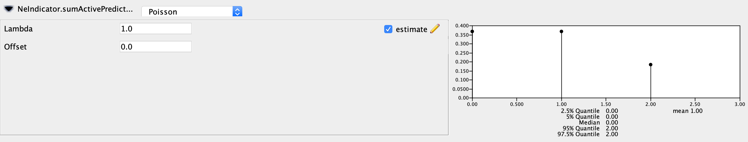
The priors that end with .sumActivePredictors denote the prior distribution on the number of active predictors. As in Bayesian Stochastic Search Variable Selection (BSSVS), we can assign an indicator variable to each predictor variable, which can be either on or off. The sumActivePredictors sets the prior on the number of predictor variables we want to be active or “on”. I recommend leaving the Poisson prior with a lambda (mean) of one so that we place more prior probability on zero or one predictor being included rather than two. Make sure to set these priors for both the NeIndicator and the migrationIndicator.
Setting up the MCMC run
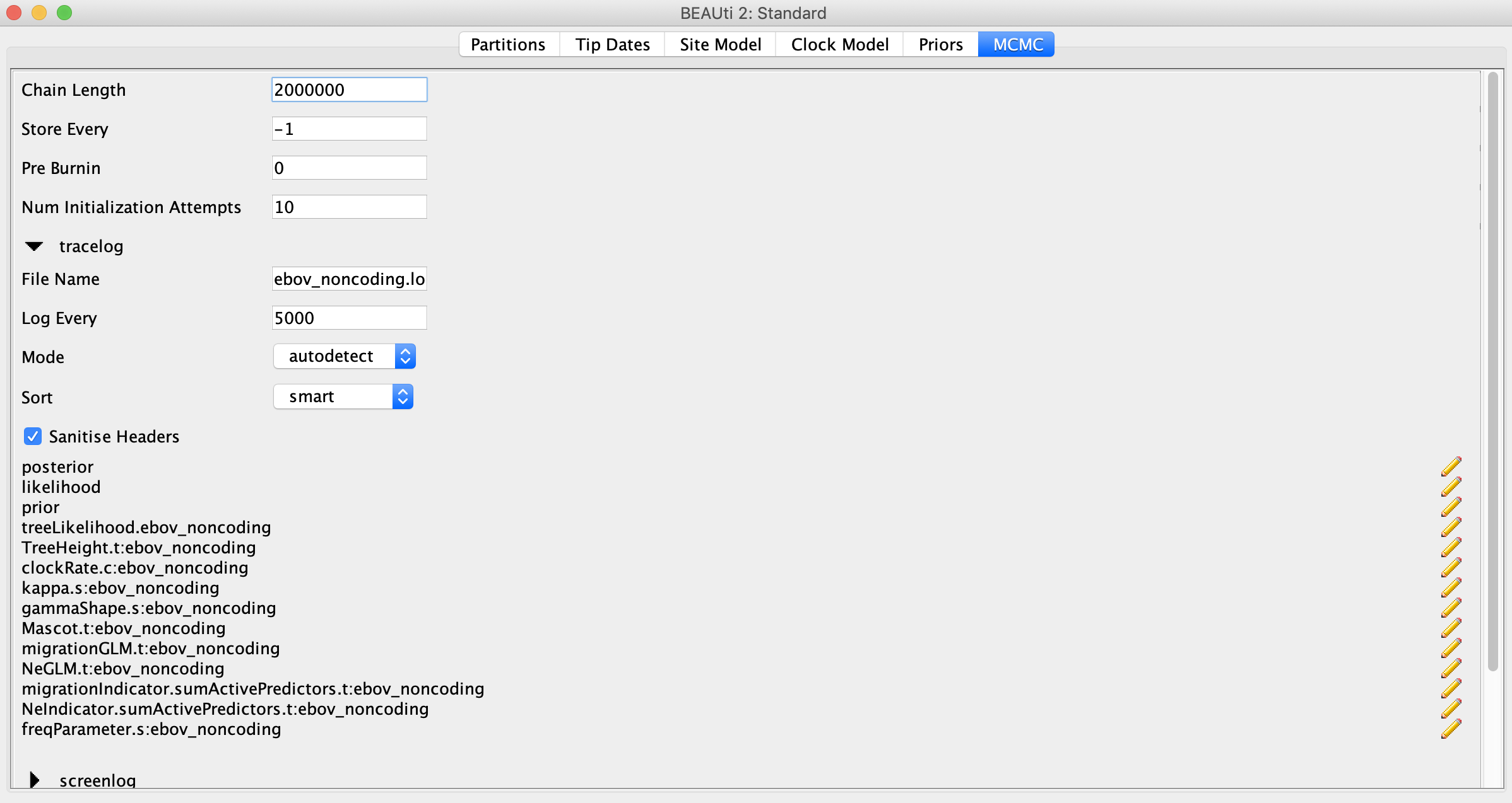
Click on the MCMC tab and set the chain length to 2 million, which should be sufficient for this small dataset. In order to have enough samples but not create log files that are too large, we can set the logEvery to 5000 under tracelog.
Finally go to File → Save to save the settings in a XML file named something like ebola_mascot_glm.xml. You can now run this XML file in BEAST.
If you cannot get BEAST to run with your XML file, you can try running my pre-cooked XML.
Visualizing spatial spread in the MCC tree
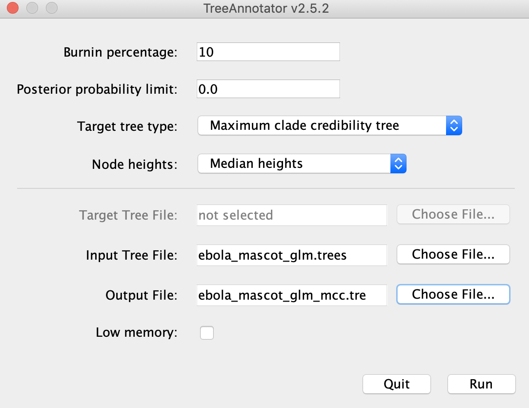
After BEAST has finished running, open TreeAnnotator. Set the Burnin percentage to 20%, select Maximum clade credibility tree for the Target tree type and select Median heights for Node heights. Select the .trees file from your BEAST run as the Input and select an output file and hit Run.
We can open the MCC tree in FigTree to visualize the reconstructed ancestral states. In each tree logging step during the MCMC, MASCOT logs the inferred probability of each node being in each possible location and the most likely location of each node. To color branches according to the most likely location, you can go to Appearance → Colour by and select max.
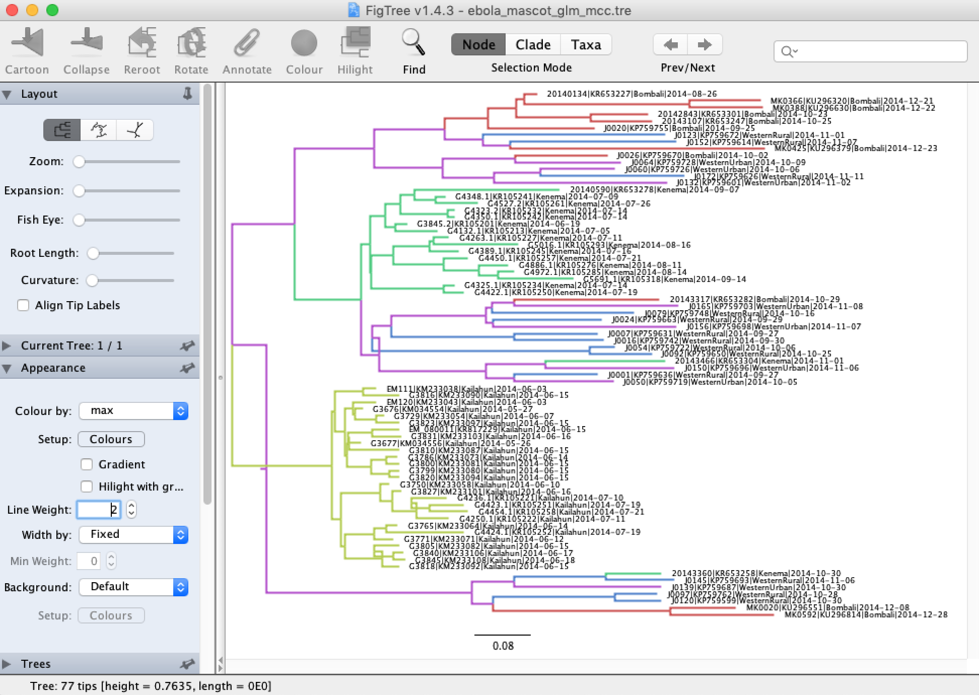
Note that the MCC tree here looks funny because we have negative branch lengths. This can happen because TreeAnnotator does not necessarily make sure that the median branch lengths are consistent when determining the MCC tree. Typically this happens when there is a high degree of uncertainty surrounding the branch lengths. Using the full EBOV genomes instead of only the non-coding sequence regions likely would have prevented this.
To view the posterior ancestral state probabilities, check the Node Labels box and then under Display select one of the locations. This displayes the inferred posterior probability of each node being in that location.
Exploring the predictors of spread
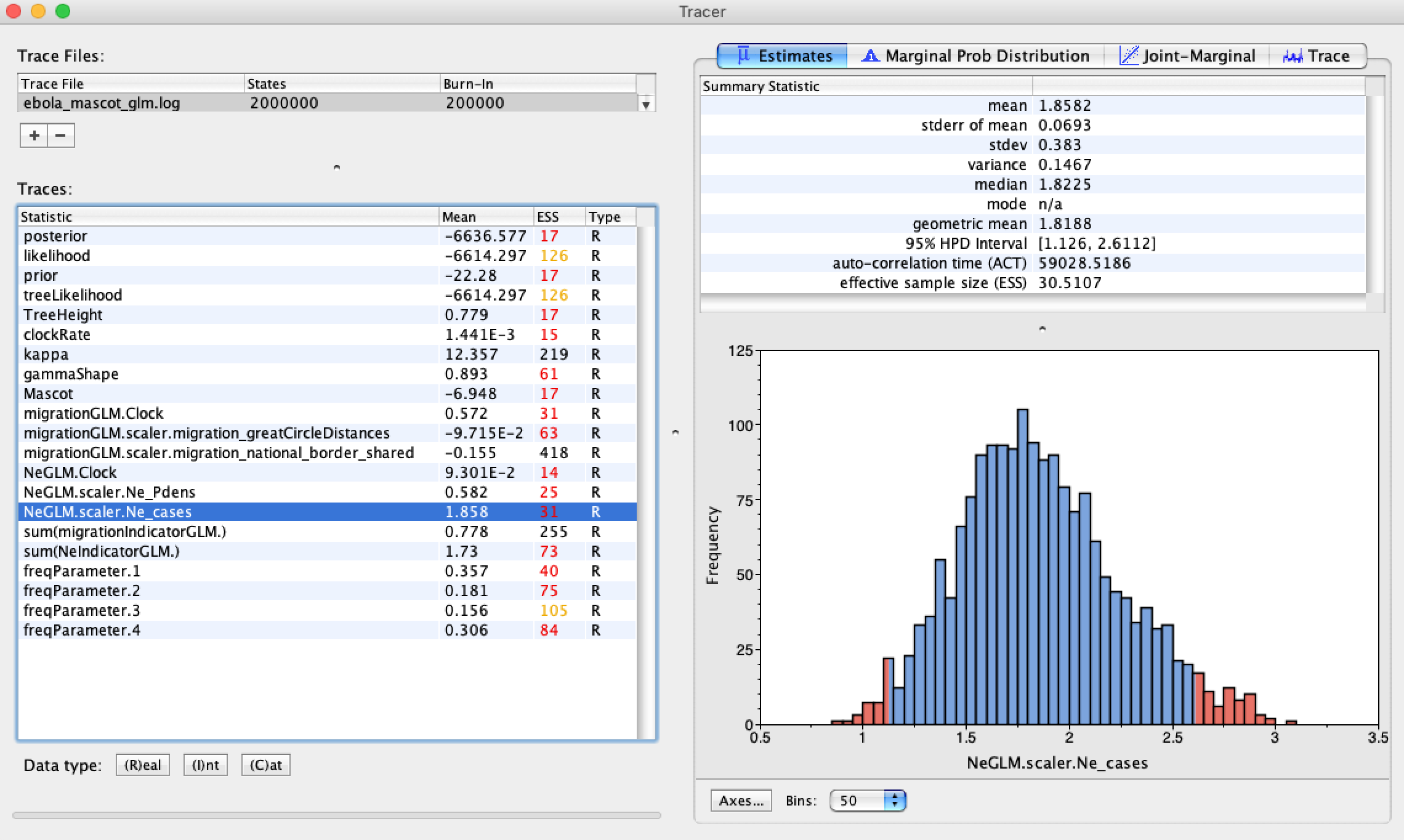
Finally, open the .log file from your BEAST run to see which of the explanatory variables proved to be good predictors of the effective population sizes and migration rates. The relevant parameter here is the scalar value associated with each predictor variable, as this gives the effect size of each predictor on the estimated parameter.
As we can see, neither of the migration rate predictors has a large effect on the migration rates. This is not necessarily surprising. As we learned, geographic distances and proximity are often poor predictors of spatial spread since they do not necessarily reflect transportation networks. You can check out the paper by Dudas et al., (2017) to see what factors predicted spatial spread for the whole Ebola epidemic. On larger spatial scales, it does appear that geographic distances become a good predictor of viral movement.
On the other hand, both the population densities and the weekly case reports are strong predictors of the effective population sizes. Thus, as we might expect, effective population sizes are positively correlated with weekly case counts.
Unfortunately, it is not possible as of now to log the actual estimated effective population sizes or migration rates estimates in MASCOT, but this will be available soon.
Acknoweledgments
This tutorial was based on a tutorial by Nicola F. Müller.