Simulating epidemics and trees with MASTER
What you will need:
-BEAST 2.5.0 or greater
-FigTree
-Python 3.6 or later with Anaconda
-Pyvolve
Stochastic simulations using MASTER
In lecture this week, we learned how the stochastic simulation algorithm (SSA) can be used to simulate stochastic epidemic dynamics and transmission trees. In this week’s tutorial, we will use Tim Vaughan’s MASTER package to simulate epidemic dynamics and trees in BEAST 2 (Vaughan and Drummond, 2013). MASTER is quite versatile and can be used to simulate stochastic dynamics under almost any continuous-time, discrete-state Markov model. Here, we will simulate epidemics and trees under a stochastic SEIR model, which extends the basic SIR model by adding an exposed compartment for infected hosts who are not yet infectious. This model is commonly used for diseases where the incubation period (i.e. the time spent in the exposed class) is not so short relative to the duration of infection that it can simply be ignored.
The goal for this week is to simulate epidemic dynamics and trees under the SEIR model, and then simulate molecular evolution along the lineages of the tree to generate mock sequence data. We will then be able to use this simulated data next week to test our implementation of the SEIR model in BEAST by seeing if we can estimate the epidemiological parameters we used in our simulations back from the phylogenetic trees!
Installing MASTER
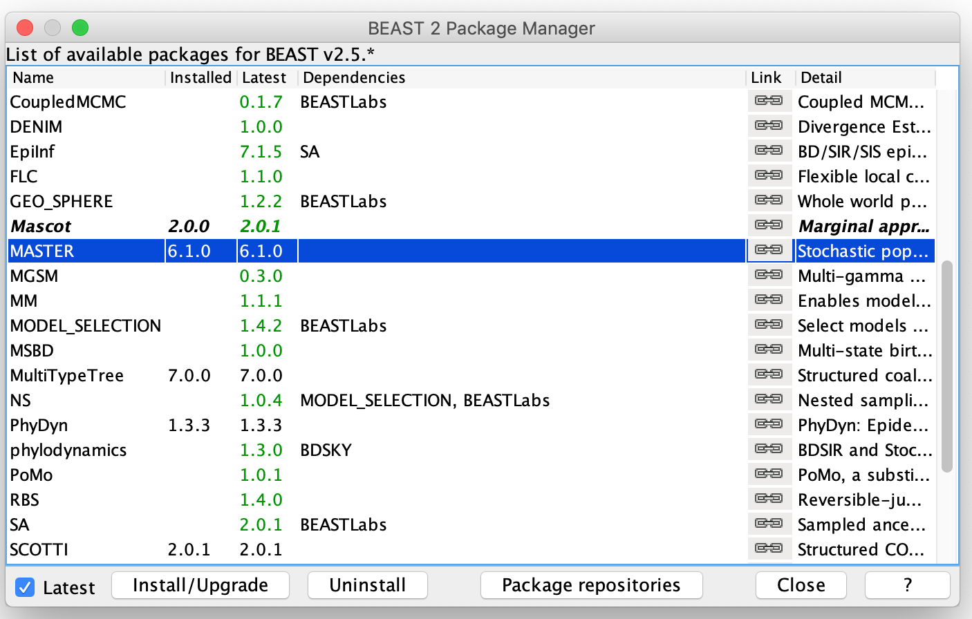
We can install the MASTER package just as we installed other BEAST add-ons using the Package Manager in BEAUTi.
Note: you may already have MASTER installed from the BDMM tutorial.
Open BEAUTi and select File → Manage packages. Select MASTER and then hit Install/Upgrade.
Specifying the MASTER XML file
First, we need a XML input file for BEAST to run our simulations. This XML file will specify the stochastic model we want to simulate under. However, unlike in previous weeks where we used BEAUTi to generate XML files, we will create this XML ourselves.
Open a blank document in your favorite text editor. The first thing we need to add is a standard XML element that lets BEAST know that this is a valid input and where to find the MASTER plug-ins. You can copy and paste the following code block directly into your XML document:
<beast version='2.0' namespace='master:master.model:master.steppers:master.conditions:master.postprocessors:master.outputs'>
</beast>
XML files have a hierarchical structure in which individual XML elements are nested within each other (each element is always surrounded by <element> tags). Within the outer BEAST element we just created, we can add a run element which tells MASTER what type of simulation we want to run.
<beast version='2.0' namespace='master:master.model:master.steppers:master.conditions:master.postprocessors:master.outputs'>
    <run spec='Trajectory'
         simulationTime='50'>

    </run>
</beast>
Here, we have set up a single simulation (called a Trajectory) with a length of 50 time units, which we will think of as days.
Within the run element, we specify our model. The population elements indicate what types of individuals are in the model. We have four types corresponding to susceptible (\(S\)), exposed (\(E\)), infected (\(I\)) and recovered (\(R\)) hosts.
Below the population elements, we set up the different types of events that can occur, which MASTER refers to as reactions. Each reaction element has both a reactionName and a rate parameter that sets the rate at which the reaction occurs. For our SEIR model there are three types of reactions: infections (i.e. transmission events), incubations and recoveries. We specify what exactly happens at each reaction event within the reaction element. For example, at a transmission event a \(S\) and a \(I\) host react to create an infected (\(I\)) host and a new exposed (\(E\)) host. Some reactions may only involve one host. For example, an incubation reaction converts an exposed (\(E\)) host into an infected (\(I\)) host:
<model spec='Model' id='model'>
      <population spec='Population' id='S' populationName='S'/>
      <population spec='Population' id='E' populationName='E'/>
      <population spec='Population' id='I' populationName='I'/>
      <population spec='Population' id='R' populationName='R'/>

      <reaction spec='Reaction' reactionName="Infection" rate="0.01">
        S + I -> I + E
      </reaction>
      <reaction spec='Reaction' reactionName="Incubation" rate="0.4">
        E -> I
      </reaction>
      <reaction spec='Reaction' reactionName="Recovery" rate="0.2">
        I -> R
      </reaction>
</model>
All of this can be copied and pasted within the run element, although don’t worry too much about constructing the whole XML right now because you can download the full version below.
A quick note on the rates, for reactions with a single type of reactant (e.g. incubations), these are the per-capita rates. MASTER will automatically multiply the rate by the total number of reactants to get the total reaction rate in the population. For reactions involving a pair of reactants (e.g. infections), the rate is scaled by the number of possible reaction pairs.
Next, we use the initialState element to set our initial conditions. We will use a total population size of 200 with 199 initially susceptible hosts and a single infected host, which are set in the populationSize elements corresponding to each population. If no population size is specified, the initial population size is assumed to be zero, so we do not need to set the initial size of the recovered population.
<initialState spec='InitState'>
    <populationSize spec='PopulationSize' population='@S' size='199'/>
    <populationSize spec='PopulationSize' population='@E' size='0'/>
    <populationSize spec='PopulationSize' population='@I' size='1'/>
</initialState>
The last thing we need to set is where the output will be saved. MASTER saves this output as a JSON file, which can easily be parsed in Python or R. Note that I’m saving the output to my Desktop but you may want to set a different location.
<output spec='JsonOutput' fileName='Desktop/SEIR_output.json'/>
The fully constructed XML file for the SEIR model is available here.
You can now run the XML file in BEAST! Open BEAST, select the SEIR-master-sim.xml file and hit Run. It should only take a few seconds for the simulation to run because our population sizes are small.
Now we would like to be able to plot the epidemic dynamics. I’ve created a plot_master_sim.py Python script that parses the JSON output file from MASTER and plots the epidemic dynamics, which can be downloaded here. You will need to have Python with Anaconda installed to run this. To plot the dynamics, run the following command from the command line in the directory where you saved the JSON output file and Python script:
python plot_master_sim.py SEIR_output.json SEIR_curves.png
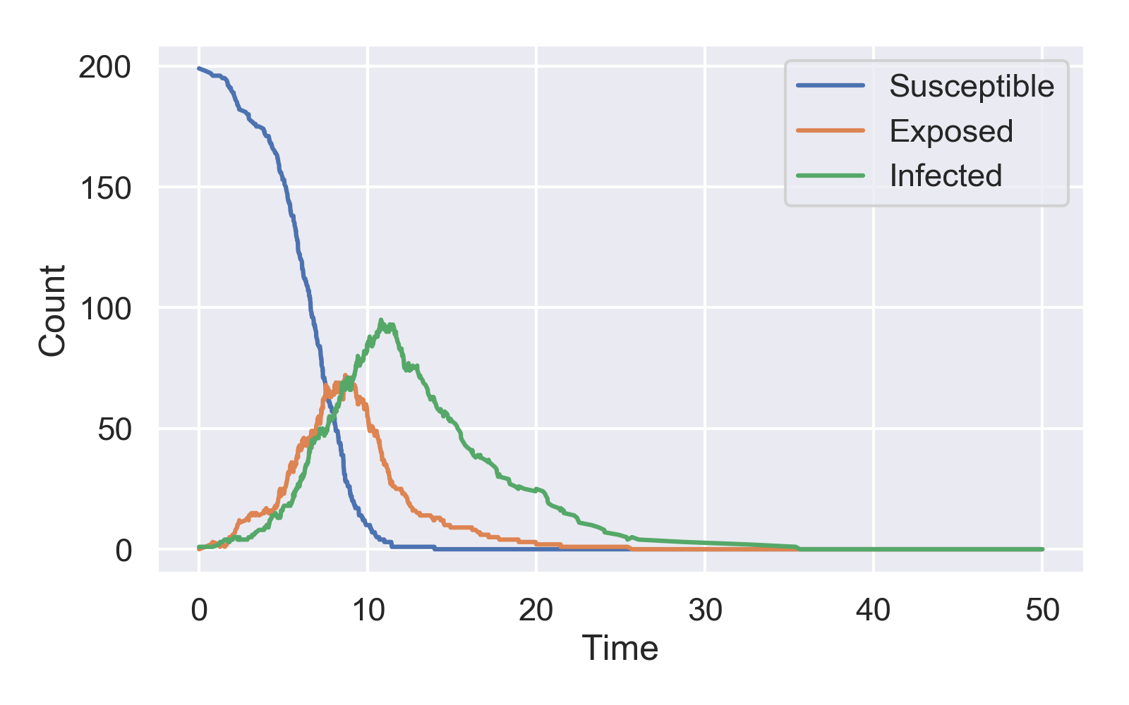
The first input argument sets the JSON file to parse and the second (optional) argument sets the name of the png file where the plot will be saved. My simulated epidemic dynamics look like this:
Simulating transmission trees with MASTER
Simulating transmission trees only requires a few changes to the XML file we just created. First, we modify the run element from <run spec='Trajectory' to <run spec='InheritanceTrajectory'. An InheritanceTrajectory is how MASTER tracks the ancestry, or inheritance, of the population including the parent-child relationships at transmission events needed to reconstruct the transmission tree. We will also set samplePopulationSizes="true" so that we continue to track the trajectory of the epidemic dynamics. The first few lines of the XML should now read like this:
<beast version='2.0' namespace='master:master.model:master.steppers:master.conditions:master.postprocessors:master.outputs'>

  <run spec='InheritanceTrajectory'
       samplePopulationSizes="true"
       simulationTime='50'>
We do not need to change the populations or reactions in the SEIR model. But we do need to make a minor tweak in the reactions to properly track the ancestry of the population.
<model spec='Model' id='model'>
      <population spec='Population' id='S' populationName='S'/>
      <population spec='Population' id='E' populationName='E'/>
      <population spec='Population' id='I' populationName='I'/>
      <population spec='Population' id='R' populationName='R'/>

      <reaction spec='Reaction' reactionName="Infection" rate="0.01">
        S + I:1 -> I + E:1
      </reaction>
      <reaction spec='Reaction' reactionName="Incubation" rate="0.4">
        E:1 -> I:1
      </reaction>
      <reaction spec='Reaction' reactionName="Recovery" rate="0.2">
        I -> R
      </reaction>
</model>
Note the :1 after the \(I\) and the \(E\) in the Infection reaction. Attaching these IDs lets MASTER know how the reactants are related: reactants and products having the same ID are assumed to have a parent/child relationship. So in our case, the newly infected \(E\) individual on the right side of the reaction will be the direct descendant of the \(I\) individual on the left side. We also do something similar for the Incubation reaction so that the \(I\) individual on the right side is the direct descendant of the \(E\) individual on the left side.
Inside the initialState we need to add a lineageSeed element to specify an individual that will seed the simulated transmission tree. This individual will be at the root of the transmission tree and can therefore be thought of as “case zero”. We will assign this individual to the infected \(I\) population:
<initialState spec='InitState'>
    <populationSize spec='PopulationSize' population='@S' size='199'/>
    <populationSize spec='PopulationSize' population='@E' size='0'/>
    <populationSize spec='PopulationSize' population='@I' size='1'/>
    <lineageSeed spec='Individual' population='@I'/>
</initialState>
Next we will add a LineageEndCondition element that adds another end condition for terminating the simulation. In this case, the simulations will end when the number of lineages in the transmission tree reaches zero, meaning that the epidemic has died off:
<lineageEndCondition spec='LineageEndCondition' nLineages="0"/>
We will also add a inheritancePostProcessor element that will process the transmission tree after the simulation is completed. To make our simulations more realistic, we will only sample a small fraction of infected hosts (20%). The pSample variable sets what fraction of the infected population we want to sample:
<inheritancePostProcessor spec='LineageSampler'
    pSample="0.2">
</inheritancePostProcessor>
MASTER includes several options for how lineages are sampled through the LineageSampler. For example, you can specify the exact number of lineages to sample using nSamples and when to sample using samplingTime variables. Check out the LineageSampler documentation for more details.
Finally, we will add an additional Nexus output file to store our transmission tree along with the JSON output file.
<output spec='NexusOutput' fileName='Desktop/SEIRTree_output.nexus'/>
<output spec='JsonOutput' fileName='Desktop/SEIRTree_output.json'/>
The fully constructed XML file for simulating transmission trees under the SEIR model is available here. You can now run the simulation in BEAST using this input XML.
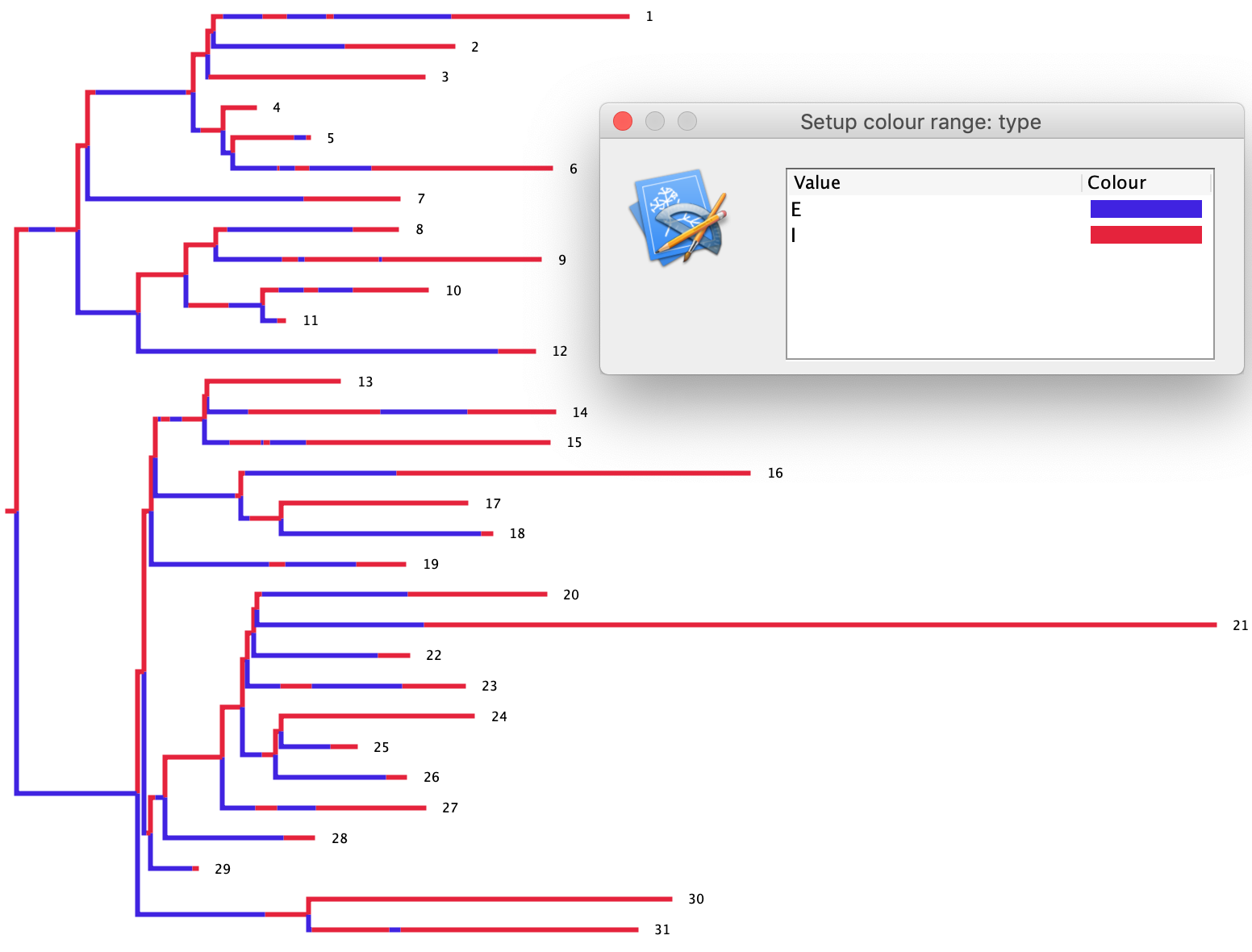
You can plot the epidemic dynamics using the plot_master_sim.py Python script as before. We can also look at the simulated transmission tree by opening the output NEXUS file in FigTree. In FigTree, click on the Appearance tab and then Colour by and select type. This will color the transmission tree according to the type of each individual lineage (\(E\) or \(I\)).
In the tree below, exposed individuals are colored blue and infected individuals red. Under the SEIR model, we know that infected individuals can transmit, but exposed individuals cannot. Thus, as a quick sanity check, we can make sure that all the parent lineages in the tree are in the infected state (red) at branching/transmission events. Fortunately, this appears to be the case, suggesting our simulations are working correctly.
Adding high and low risk groups to the SEIR model
To make things more interesting, we will add risk structure to our SEIR model with infected hosts that transmit at either high and low rates. We will simulate epidemic dynamics and transmission trees under this model, and then use these trees to simulate the sequence data we will use next week to test BEAST. We will then be able to check whether we can accurately estimate the basic reproductive number \(R_{0}\) as well as the relative transmission rates from high and low risk individuals.
We need to make a few changes in the model element in order to implement this model. First, we will split the infected population into low-risk \(I_{l}\) and high-risk \(I_{h}\) infected subpopulations.
We also need to split the infection, incubation and recovery reactions into two types of reactions corresponding to the high and low risk groups. For the infection reactions, we will set the transmission rate for the InfectionHigh reaction to five times higher than the transmission rate for the InfectionLow reaction to generate some transmission heterogeneity between risk groups.
The incubation reactions require a little more thought. Previously, we had the incubation rate for the \(E\) to \(I\) reaction set to 0.4. I propose that we follow the “80/20” rule of infectious disease epidemiology and let 80% of exposed hosts incubate into the low risk group and the other 20% incubate into the high risk group. How can we specify this in terms of the reaction rates? We can set the IncubationLow reaction rate four times higher than the IncubationHigh rate. So we will set the IncubationLow reaction rate to 0.32 and the IncubationHigh rate to 0.08 so the incubation rates still sum to an overall incubation rate of 0.4. Now we can think of the two types of incubations as competing or dueling reactions, so the relative probability that an exposed individual incubates into the low risk group will be \(\frac{0.32}{0.32+0.08} = 0.8\), and for the high risk group \(\frac{0.08}{0.32+0.08} = 0.2\).
We will leave the recovery rates equal for high and low risk individuals.
The overall model element should now look like this:
<model spec='Model' id='model'>
      <population spec='Population' id='S' populationName='S'/>
      <population spec='Population' id='E' populationName='E'/>
      <population spec='Population' id='Il' populationName='Il'/>
      <population spec='Population' id='Ih' populationName='Ih'/>
      <population spec='Population' id='R' populationName='R'/>

      <reaction spec='Reaction' reactionName="InfectionLow" rate="0.005">
        S + Il:1 -> Il + E:1
      </reaction>
      <reaction spec='Reaction' reactionName="InfectionHigh" rate="0.025">
        S + Ih:1 -> Ih + E:1
      </reaction>
      <reaction spec='Reaction' reactionName="IncubationLow" rate="0.32">
        E:1 -> Il:1
      </reaction>
      <reaction spec='Reaction' reactionName="IncubationHigh" rate="0.08">
        E:1 -> Ih:1
      </reaction>
      <reaction spec='Reaction' reactionName="RecoveryLow" rate="0.2">
        Il -> R
      </reaction>
      <reaction spec='Reaction' reactionName="RecoveryHigh" rate="0.2">
        Ih -> R
      </reaction>
</model>
In the initialState element we now need to specify in which risk group the epidemic starts. We will seed the epidemic in the high risk group to give the epidemic a higher probability of taking off:
<initialState spec='InitState'>
    <populationSize spec='PopulationSize' population='@S' size='999'/>
    <populationSize spec='PopulationSize' population='@E' size='0'/>
    <populationSize spec='PopulationSize' population='@Il' size='0'/>
    <populationSize spec='PopulationSize' population='@Ih' size='1'/>
    <lineageSeed spec='Individual' population='@Ih'/>
</initialState>
Note that we now set the initial susceptible population size to 999, so that we get a larger epidemic and transmission tree. Having a larger tree will ensure that there’s enough information in the tree to estimate differences in transmission rates between risk groups next week.
We can leave the lineageEndCondition and inheritancePostProcessor elements alone. We will however modify the output to generate two different NEXUS trees. The first tree will include all the information we had before, including when lineages change states along branches. These changes are represented in the NEXUS tree as nodes with only a single child node in a different state than the parent. We want to keep this information for visualizing the simulated transmission trees but these single child nodes WILL BREAK the coalescent methods we will use next week in BEAST, which expect tree nodes to always be bifurcating with two children. We can therefore output a second NEXUS tree with the collapseSingleChildNodes variable set true so that we also have a tree that we can input into BEAST.
<output spec='NexusOutput' fileName='Desktop/SEI2RTree_output.nexus'/>
<output spec='NexusOutput' fileName='Desktop/SEI2RTree_TreeForBEAST.nexus'
    collapseSingleChildNodes='true'/>
<output spec='JsonOutput' fileName='Desktop/SEI2RTree_output.json'/>
The fully constructed XML file for simulating transmission trees with high and low risk groups is available here. You can run the simulation in BEAST using this input XML.
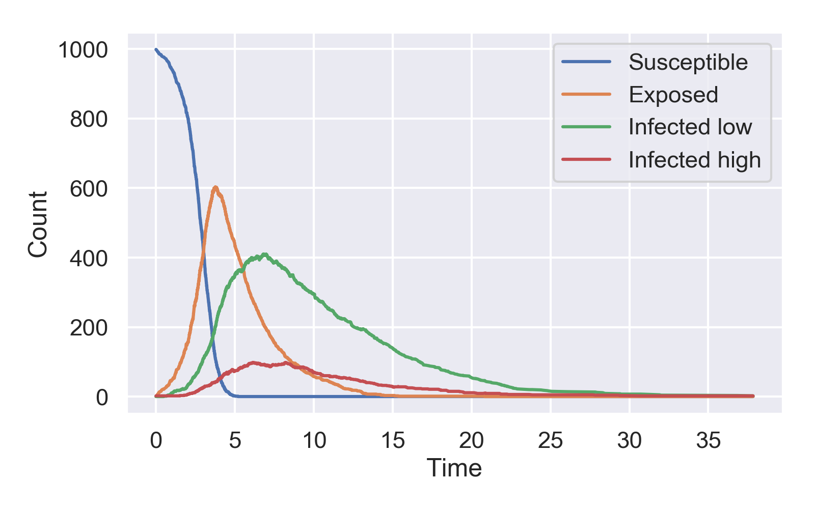
Plotting the epidemic dynamics using the plot_master_sim.py script, we see that there are many more low risk than high risk infected individuals as expected:
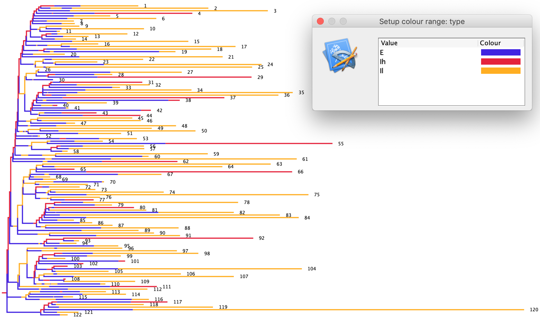
Open the SEI2RTree_output.nexus tree in FigTree. To color the transmission tree click on the Appearance tab, then Colour by and select type. In the transmission tree plotted below high risk individuals are colored red and low risk individuals orange. As another sanity check, we can check that most of the transmission events derive from high risk individuals since they transmit rate at a 5X higher rate than low risk individuals. This appears to be the case in my simulated tree:
Because these are stochastic simulations, there will be stochastic variation in the size of the epidemic and the resulting transmission tree between runs. We would like a tree that is large enough to allow for estimation of our epidemic parameters but not so large that BEAST will take a long time to run. I recommend aiming for a tree with between 100 and 200 sampled lineages. If your tree is outside this range, you can always run another simulation in BEAST using the same XML file.
Advanced: Simulating sequences using Pyvolve
To finish up, we would now like to simulate sequence data that we can use to test BEAST next week. We will use the pyvolve Python package to simulate molecular evolution along the branches of the transmission tree we just simulated.
You will first need to install pyvolve, which in turn requires Biopython. If you would rather not install all these packages feel free to just follow along and download the pre-cooked sequences I simulated using the link below. If you want to follow along and run the simulations yourself, you can install pyvolve from the command line using conda:
conda install -c bioconda pyvolve
WARNING: Older versions of pyvolve (<1.1) no longer seem to work with Biopython. If you have an older version of pyvolve installed, you can uninstall pyvolve and then re-install the new 1.1 version using pip:
conda remove pyvolve
pip install pyvolve==1.1
Please also download my sim_tree_seqs.py Python script and the baltic package, which we will use to process our trees:
You can run the sim_tree_seqs.py script like this:
python sim_tree_seqs.py SEI2RTree_TreeForBEAST.nexus
Make sure the first argument after the python script is the TreeForBEAST nexus file. This script returns two files. The first is a FASTA file with the simulated sequences and the second is a new tree file with the tips relabeled to correspond to the sequence names in the FASTA file. The tips and sequences are relabeled so that the sampling times and tip states (high or low risk group) are in the names, and so can easily be parsed later.
Now let’s take a look inside the sim_tree_seqs.py script to see what is going on. After relabeling the sample names, we define the parameters we will use to simulate the sequence data:
"User defined params"
mut_rate = 0.005 # rate per day
freqs = [0.25, 0.25, 0.25, 0.25] # equilibrium nuc freqs
seq_length = 2000 # length of sim sequences
kappa = 2.75 # kappa parameter in HKY model
Here we have set the mutation rate, nucleotide frequencies, sequence length and the kappa parameter (transition vs. transversion rate) of the HKY model we will use to simulate our sequences.
We then read in our tree using pyvolve. The branch lengths in the tree get rescaled by the mutation rate so that the mutation rate becomes one per unit of tree time.
"Read in phylogeny along which Pyvolve should simulate"
my_tree = pyvolve.read_tree(file = relabledTreeFile, scale_tree = mut_rate) #Scale_tree sets absolute mutation rate
Now we need to set up our nucleotide substitution model. Here we will use a HKY model with the kappa parameter and equilibrium state frequencies we defined above:
"HKY model with kappa"
nuc_model = pyvolve.Model( "nucleotide", {"kappa":kappa, "state_freqs":freqs})
Next we will set up a Partition object for our sequences. Pyvolve makes it possible to set up different partitions that can be used to evolve sites in different partitions under different models of molecular evolution, but for our purposes we will assign all sites to a single partition:
"Define a Partition object which evolves set # of positions according to my_model"
my_partition = pyvolve.Partition(models = nuc_model, size = seq_length)
Now we can create an instance of the Evolver class to evolve our sequences in my_partition along our tree in my_tree:
"Define an Evolver instance to evolve a single partition"
my_evolver = pyvolve.Evolver(partitions = my_partition, tree = my_tree)
Finally, we will evolve our sequences along the tree using my_evolver.
"Evolve sequences with custom file names"
my_evolver(ratefile = "sim_ratefile.txt", infofile = "sim_infofile.txt", seqfile = fastaFile)
The simulated sequences will be saved to the fastaFile we defined above. You can download the sequences I simulated here if you did not install or run pyvolve yourself.
That is pretty much all for this week. Next week we will see if we can estimate the SEIR model parameters back from the simulated trees and/or sequence data in BEAST. In the meantime, you can always set up a BEAST run (as in week 3) to see if you can reconstruct the tree and estimate the molecular evolutionary parameters we simulated under.
References and Acknowledgments
This tutorial was largely based on earlier tutorials by Tim Vaughan on the MASTER Wiki.