Fitting SIR models to phylogenies using PhyDyn
What you will need:
-BEAST 2.5.*
-Tracer 1.7.0 or greater
-FigTree
Important note: Since originally writing this tutorial in 2020, many BEAST class names have changed between BEAST 2.5.* and newer 2.7.* versions. To ensure that the XML templates provided here work correctly, please use an older 2.5.* version available to download here. I tested this on April 1st, 2024 with BEAST v. 2.5.2 and PhyDyn v. 1.3.3 and everything seemed to work correctly.
Phylodynamic inference using PhyDyn
PhyDyn is a package that allows a wide class of SIR-type epidemiological models to be fit to pathogen phylogenies in BEAST 2. Epidemic models are specified as a system of ordinary differential equations (ODEs), which are numerically integrated within BEAST to give trajectories of population variables such as the number of susceptible or infected individuals. The likelihood of a given phylogeny is then computed under the very general structured coalescent framework of Volz (2012) that we discussed in lecture. PhyDyn uses a special syntax to allow the epidemic models to be specified through an input XML file for BEAST. The appropriate structured coalescent model is then specified via two matrices that govern the birth rates (F matrix) and migration rates (G matrix) of lineages between populations.
We will implement a SEIR model with transmission heterogeneity (high and low risk groups) in PhyDyn. This is the same model we used to simulate transmission trees using MASTER in last week’s tutorial, which will allow us to test our implementation of the model in PhyDyn by checking to see if we can estimate the true epidemiological parameters back from the simulated phylogenies. Once we are sure our model is working correctly, we will then apply it to real SARS-CoV-2 sequences from Washington state to estimate key epidemiological parameters for Covid-19 such as \(R_{0}\) and the extent of transmission heterogeneity.
Installing PhyDyn
We can install PhyDyn just as we installed other BEAST add-ons using the Package Manager in BEAUTi.
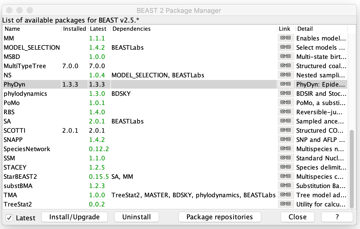
Open BEAUTi and select File → Manage packages. Select PhyDyn and then hit Install/Upgrade.
Specifying the SEI2R model in PhyDyn
To expedite things, we’ll start with a XML template that already has the SEI2R model specified in the syntax of PhyDyn, which we will walk through together below. Note that this template does not contain any data such as a sequence alignment or phylogenetic tree. We will add our simulated data to this XML file after we set up the model.
Download the SEI2R XML template and open it in your favorite text editor.
First, let’s have another look at the ordinary differential equations for the SEI2R model:
\[\begin{eqnarray} \frac{dS}{dt} & = & - (\beta I_{l}l + \tau \beta I_{h}) S \\ \frac{dE}{dt} & = & (\beta I_{l}l + \tau \beta I_{h}) S - \eta_{l} E - \eta_{h} E \\ \frac{dI_{l}}{dt} & = & \eta_{l} E - \gamma I_{l} \\ \frac{dI_{h}}{dt} & = & \eta_{h} E - \gamma I_{h} \\ \frac{dR}{dt} & = & \gamma (I_{l} + I_{h}) \end{eqnarray}\]In this model there are two infectious classes for high risk \(I_{h}\) and low risk \(I_{l}\) individuals. We will use the parameter \(\tau\) to determine how much more infectious high risk individuals are than low risk individuals (\(\tau = \frac{\beta_{h}}{\beta_{l}}\)). Exposed individuals incubate into the low risk class at rate \(\eta_{l}\) and the high risk class at rate \(\eta_{h}\). Both low and and risk infected hosts recover at rate \(\gamma\).
Now we need to translate this model into the ODE syntax of PhyDyn. We do this in the model XML element which in turn has matrixeq elements to specify the rates at which individuals move between compartments in the model. Each matrixeq has an origin and destination input variable that determines which compartments individuals move between.
Each matrixeq element also has a type variable, which can be set to a birth, death, migration or nondeme event. Births correspond to the addition of new lineages through birth or transmission events and are analogous to the elements of the \(F\) matrix we saw in lecture. Migration events correspond to the movement of lineages between populations in absence of a birth or transmission event, and are analogous to the elements of the \(G\) matrix we saw in lecture. Death events remove lineages, such as when an infected individual recovers. Nondeme types are compartments for non-infected hosts like \(S\) and \(R\) in which pathogen lineages cannot reside.
Note that by setting the birth and migration types in the model, we are fully specifying the structured coalescent model under which the likelihood of the phylogeny will be computed. Death and nondeme events do not directly enter into the structured coalescent model but still need to specified in the ODE model because they can influence the dynamics of other population variables such as \(S\).
You can find much more information on how models are specified on the PhyDyn wiki page. The fully specified SEI2R model appears as the following code in the template XML:
  <model spec='PopModelODE' id='seirmodel' evaluator="compiled"
       popParams='@initValues' modelParams='@rates'>

    <matrixeq spec='MatrixEquation' type="nondeme" origin="S">
            - (beta*Il + beta*Ih*tau) * S
    </matrixeq>

    <matrixeq spec='MatrixEquation' type="migration" origin="E" destination="Il">
      E*eta_l
    </matrixeq>

    <matrixeq spec='MatrixEquation' type="migration" origin="E" destination="Ih">
      E*eta_h
    </matrixeq>

    <matrixeq spec='MatrixEquation' type="birth"  origin="Il" destination="E">
      beta*Il
     </matrixeq>

    <matrixeq spec='MatrixEquation' type="birth"  origin="Ih" destination="E">
      beta*Ih*tau
     </matrixeq>

    <matrixeq spec='MatrixEquation' type="death" origin="Il">
      gamma*Il
    </matrixeq>

    <matrixeq spec='MatrixEquation' type="death" origin="Ih">
      gamma*Ih
    </matrixeq>

    <matrixeq spec='MatrixEquation' type="nondeme" origin="R">
      gamma*(Il + Ih)
    </matrixeq>
  </model>
Next we need to set the parameters in our ODE model in the rates element. We will not estimate \(\eta_{h}\), \(\eta_{l}\) and \(\gamma\), so I have set these parameters to the values we used last week to simulate the transmission trees in MASTER. We will however infer \(\beta\) and \(\tau\). Since these are estimated parameters, we will need to initialize them below as part of the MCMC. The @ symbol in front of their names indicates that this is a reference to another variable we will specify elsewhere in the XML.
  <rates spec="ModelParameters" id='rates'>
    <param spec='ParamValue' names='eta_h' values='0.08'/>
    <param spec='ParamValue' names='eta_l' values='0.32'/>
    <param spec='ParamValue' names='gamma' values='0.2'/>
    <param spec='ParamValue' names='beta' values='@beta'/>
    <param spec='ParamValue' names='tau' values='@tau'/>
  </rates>
In order to compute the likelihood of our tree under the SEI2R model, we need to be able to solve or numerically integrate the ODEs specified above to obtain the trajectories of the population variables. The trajparams element specifies how to solve the ODEs. We will use the classicrk method, which is the very old and venerable Runge-Kutta method. Here we will use a fixed number of integration time steps (400) starting at time t0. We also need to set the initial conditions in the trajparams element. Here I used the same values we used in our simulation last week. Note that for \(I_{h}\), I am passing in a reference to another variable @initI0, giving us the option to estimate the initial number of infections in the high risk group below.
  <trajparams id='initValues' spec='TrajectoryParameters' method="classicrk"
              integrationSteps="400" t0="-0.001">
      <initialValue spec="ParamValue" names='S' values='999.0'  />
      <initialValue spec="ParamValue" names='E' values='0.0'  />
      <initialValue spec="ParamValue" names='Il' values='0.0'  />
      <initialValue spec="ParamValue" names='Ih' values='@initI0'/>
      <initialValue spec="ParamValue" names='R' values='0.0'  />
  </trajparams>
There is a lot of other stuff going on in the XML template, but so we don’t get lost in the weeds I just want to draw your attention towards a few other features that you may wish to modify.
First, let’s look inside the state element, which determines what parameters are included as state variables in the MCMC, and will therefore be estimated. Included among these are the three parameters in our epidemic model that we will infer. Its possible to set lower and upper limits on each parameter as well as their initial parameter values between the > and < arrows.
  <!-- Epi params in SEI2R model -->
  <parameter id="initI0" lower="0.0" upper="100" name="stateNode">1.0</parameter>
  <parameter id="beta" lower="0.0" upper="Infinity" name="stateNode">1.0</parameter>
  <parameter id="tau" lower="-Infinity" upper="Infinity" name="stateNode">5.0</parameter>
Further down in the XML there is the distribution element, in which we specify the priors and the posterior distribution we would like to sample from. Among the priors we can find the prior on our three estimated parameters:
  <prior id="initI0prior" name="distribution" x="@initI0">
    <LogNormal id="LogNormal:initI0" meanInRealSpace="true" M="0" S="1" name="distr" />
  </prior>
  <prior id="tauPrior" name="distribution" x="@tau">
    <LogNormal id="LogNormal:tau" meanInRealSpace="true" M="5.0" S="1" name="distr" />
  </prior>
  <prior id="betaPrior" name="distribution" x="@beta">
    <LogNormal id="LogNormal:b" meanInRealSpace="true" M="5.0" S="1" name="distr" />
  </prior>
Below the distribution element, we can find the operator elements. The operators determine how BEAST proposes new values of the estimated parameters in the MCMC. Here we are using random walk operators to propose new values of \(\beta\) and \(\tau\) from a Gaussian (Normal) distribution and an UpDown operator which will simultaneously increase \(\beta\) while decreasing \(\tau\). Note that I have commented out the operator on the initial number of infections initI0, which means BEAST will never propose new values for this parameter, effectively fixing this parameter at its initial value. This is a useful trick to know if there’s parameters we decide we would rather not estimate.
    <!-- Operators on epi model params -->
    <operator id="rwoperator:beta" spec="RealRandomWalkOperator" windowSize="0.150" parameter="@beta" useGaussian='true' weight="1" />
        <operator id="rwoperator:tau" spec="RealRandomWalkOperator" windowSize="0.1" parameter="@tau" useGaussian='true' weight="1" />
        <operator id="updownBetaTau" scaleFactor="0.75" spec="UpDownOperator" weight="2.0">
                <up idref="beta"/>
                <down idref="tau"/>
        </operator>
    <!-- <operator id="rwoperator:initI0" spec="RealRandomWalkOperator" windowSize="1.50" parameter="@initI0" useGaussian='true' weight="1" /> -->
Testing the SEI2R model in PhyDyn
Now that we have the model set up, let’s test it using the sequence data and tree we simulated last week. First we will need to add the simulated sequences and the sampling dates to the XML template. BEAST expects these to be in a very particular format, so the easiest way to add them is to first create a new XML file in BEAUTi and then copy and paste the sequence alignment and sampling dates from the BEAUTi-generated XML to our template XML.
Open BEAUTi and load in the sequences you simulated last week using Import Alignment. Alternatively, you can download and import the sequences I simulated here.
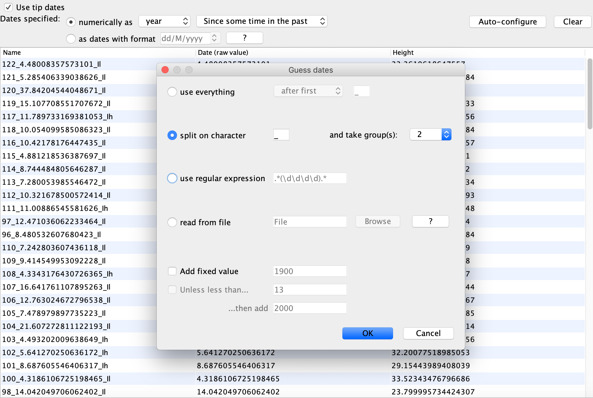
Navigate to the Tip Dates, select Use tip dates and click Auto-configure. To parse the tip dates from the sample names in the Guess Dates menu, select split on character with a underscore, and then take group 2:
That is all we need to do here because we will not be setting up our analysis in BEAUTi. Just save the XML file using a name such as SEI2R_simSeqs_beauti.xml.
Open the XML file you just created in BEAUTi and you should see a data element near the top of the file with the sequence alignment. It should look like this:
<data id="SEI2RTree_sim_TreeForBEAST" name="alignment">
      <sequence id="seq_100_4.3186106725198465_Il" taxon="100_4.3186106725198465_Il" totalcount="4" value="AGGGAGCTCCTTGAAAGTGCATGTACTGACACAATCGATGATCGCTGCTTCTAGGCTGGCAGGAGCTCATAAAAGAACAAATGAGTCTTCAGAGCTCACATTTATTTTATGGGCTTCTTCACTGGGTCTGAGGGTGGTAGCCCCAGAAGAACGCTGGGGGCCCTACTTTGATTTGGGTCAGATATACAAGATCCAGGGTTTTAACGATTTGACGTATGGTTGCGCCACCAGGGTGAGTGAGTAAGCGTGAATAATTCGTTCTTAGCATTACATCTGAAGAAGCAGGGACTAAAGCCGACATGAACAACGTAGTAAGAGGTCAATGTCTTGGGAATGTTCATCAACAGGGCTCTTCAGAAAAAGAGTTTCGTCGCCGCGACACCATACTGTCCCGTAGCGACATGTGCAAGTAGGTTTCCCGCGTTGTACCGACCCTTTATCTATGCATGCTAGCTGGCTTCATTACTCACCAAATCAGGGATAATCGCATGGCAGTTCGGTCTCACGCACAAGGTGGGAGCTACTCAATATTAGCATGATCTTTCAGGCGAGAATATCCGCACTTTGGTCCCGAAGTTTGACAACTAGGAATGCTGAGTTCCACTTTAATAGTGAAGACAGTTGCGTGACTGAAACACTCACCTTGGGCATTCGACCGTAGGATGTCACTTAGGGAACCCACGAGCACCTTTTACGTCGTGAATTCAGGCGAGCATGGTTACAGCCTGGTTAGACCACCGGCATCTGGCTCTCATATGCAGACTGGAAGCCTAAATAATCCTCCGTCTAGCTTACTAAATACGTTTACCTGAATAATGCCACGTATTTCGCGGACATTCAGATATGGCTACATCGGCCTTGAGAACGGGTGGGGGAATTACCGGTTCATAGCGTCAACTATGGGATTAGCCCAAATTATGGGCGAGCTGCCATCGTCACATCAATCTAGATAAACACATACCCAGGGAATCACGTGGAAAGAGCTAGGAGAGTAAAAGCCCGGCTAGCGCCTCCCATTGGACGACACACTTCGTAACGGTAGCATCTCTCAGAGACTAGCTACCGCCTCCTCCTACGAACGCCCTGTCTCTCCTGCCCCGCGGATTTGAGCGGCTCTGGCAATCGAATCGGAGTCGATGTTGTACACTTCCAGAAATGACGTGGCCGTCGTCAAACCCCGCGTTAGTGTGCGATCGCCTAATCACAACGGAGAGCCTCTGCCTTTCACGTCGCGCCATAGCTCAACACTGATGCCTCACTTGCGGTGAATCGCGCTCAACGGGATGGTCTCTCGGACTAGCCTAACTCAGACCTGAGCATCATGTAATGGGGGAAGCTGACGATCAAGGATGGTGAGGTATGCGCTAAAACTATGATCGTCAATATCATATACAGTGGCCAAAGGGCCACGGGAGCAGCATTGTCCATCTTTCACCGTACTCCGGTCGCGAACCTCCGGACCGACTTTGGCCTAATTTCTCGAATTTACCAAAAAGAATATCTCACAACTCCCCTTAGATTTGCTATAAGCGTGCGTTTTTCGGGGAATAACGAGCATACAGTGCTCGTGGACTCTCTTTGCTGACGGGTTTAACACTAACTTCCGAGTTACGTCACGCGCTTCATTGTAGCGATAGGTCAGGGATGGTCTGGCACCACGGTAAGTTAGTTGTACAAGCTTAACTTCGCTGGATGATACCTTTTACGGAGGGTTATCGCGTAGAATACACCTCACTACTGTCATTTGCCACAGTTTCCAGTTATAGTTCACCCAGTCCCGCTCTACCTTCACATGTAACGCAGAGCCGCAGAAACGCAATCGTCACCGTCAACGATGAGACATCTTTCATTTGAATACTGTAAATCAGTATTAGATGGATGGAAAGTCGCTACAGGTTACGACAGCCAAGGCGCTGAAGAATCAACGACCTGGGCCGGGAGTCCTACCGCACACGGACTTAAGGACGGCAACGGGCACAAGTTTAGGCTCACGGGTCAGA"/>
      <sequence id="seq_101_8.687605546406317_Ih" taxon="101_8.687605546406317_Ih" totalcount="4" value="AGGGAGCTCCTTGAAAGTGCATGTTCTGACACAATTGACGATCGCTGCTTCTAGGCTGGCAGGAGCTCGTAAAAGAACAAATGAGTCTTCAGCGCTTACATTTATTTTATGGGCTTCTTCACTGGGTCTGAGGGTGGTAGCCCCAGAAGAACGCTGGGGACCCTACTTTGATTTGGGTCAGAAATACAAGATCCAGGGTTTTAACGATTTGACGTATGGTTGCGACACCAGGGTGAGTGAGTAGGCGTGAATATTTCGTTCTTAGCATTACATCTGAAGAAGCAGGGACTAAAGCCGACATGGACAACGTAGTAAGAGGTCAATGTCTTGGGAATGTTCATCAATAGGGCTCTTCAGAAACAGAGTTTCGTCGCCGCGACACCATACTGTCCCGTAGCGACATGTGCAAGTAGGTTTCCCGCGTTGTACCGACCCATTGTCTATGCATGCTAGCTGGCTTCGTTACTCACCAAATCAGGGATAATCGCATGGCAGTTCGGTCTCACGCACAACGTGGGCGCTACTCAATATTAGCATGATCTTTCAGGCGAGAATATCCGCACTTTGGTCCCGAAGTTTGACAACTAGGAATGCTGAGTTCCACTTTAATAGTGAAGACGGTTGCGTGACTGAAACACTCACCTTGGGCATTCGACCGTAGGATGTCACTTAGGGAACCCACGAGCACCTTATACGTCGTGAGTTCAGGCGAGCATTGTTACAGCCTAGTTAGACCACCGGCATCTGGCTCTCATATGCAGACTGGAAGCCTAAAAAATCCCCCGTCTAGCTCACTAAATACGTTTACCTGAATAATTCCACGTGTTTTGCGGACATTCAGATATGGCTACATCAACCTTGAGAACGGGTGGGGGAATTACCGGTTCATAGCGTCAACTATGGGATTAGCCCAAATTATGGGCGAGCTGCCATCGTCACATCAATCTAGATGAACACACACCCAGGGAATCACGTGGAAAGAGCTAGGGGGGTAAAGGACCGGCTAGCACCTCCCATTGGATGACACACTTCGTAACGGTAGCATCTCTCAAAGACTAGCTACCGCCTCCTCCTACGAACGGCCTGTCTCTCCTGCTCCGCGGATTTGAGCGGCTCTGGCAATCGAATCGGAGTCGATGTTGTGCACTTCCAGAAATGACGTGGCCGTCGTCAAAGCACGCGTTAGTATGCGATCGCCTAATCACAGCGGAGAGCCTCTGCCTTTCAGGTCGTGCCTTAGCTCAACACTGATGCCTCACTAGCGGTGAATCGCGCTCAAGGGGATGGTCTCTCGGACTAGCCTAACTCAGACCTGAGTATCATGTAATGGGGGAAGCTGACGATCAAGGATGGTGAGGTATGCGATAAAACTTTGATCGTCAATATCATATACAGCGGCCAAAGGGCCACGGGAGCAGCATTGTCCATCTTTCACCATACTCCGGTCGCGAACCTCCGGACCGACTTTGGCTTAATTTCTCGAATTTACCACAAAGAATATCTCACAACTTCCCTTAGATTTACTATGGGCGTGCGTTTTTCGGGGAGTAACGAGCATACAGTGCTCGTGGACTCTCTTTGCTGACGGGTTTAACACTAACTTCCGAGTTACGTCACGCGCTTCATTGTAGCGCTAGGTCAGGGATGGTCTGGCACCACGGTAAGTTAGTTGTACAAGCTTAACTTCGCTGGATGATACCTTTTACGCAGGGTCATCGCGTAGAATACACCTCACTACTGTCATTTGCCACAGTTTCCAGTTATAGTTCACCCAGTCCCACTCTACCTTCACATGTAACGCAGAGCCGCTGAAACGCAATCGTCACCGTCAACGATGAGACATCTTTCATTTGAATACTGTAAATCAGTGTTAGATGGATGGAAAGTCGCTACGGGTTACGACAGCCAAGGCGCTGAAGAATCAACGACCTGGGCCGGGAATCCTACCGCACACGGAATTAAGGACGGCAACGGGCACAAGTTTAGGCTCAGGGGTCAGA"/>
Copy all the sequence elements in the alignment between the enclosing <data> element tags and paste them into the currently empty data element in the template XML for PhyDyn:
<data id="sequences" name="alignment">

</data>
Next, we need to copy the sampling dates into our template. Find the date TraitSet in the BEAUTi generated XML, which should look like this:
<trait id="dateTrait.t:SEI2RTree_TreeForBEAST" spec="beast.evolution.tree.TraitSet" traitname="date" value="122_4.48008357573101_Il=4.48008357573101,121_5.285406339038626_Il=5.285406339038626,120_37.84204544048671_Il=37.84204544048671,119_15.107708551707672_Il=15.107708551707672,117_11.789733169381053_Ih=11.789733169381053,118_10.054099585086323_Il=10.054099585086323,116_10.42178176447435_Il=10.42178176447435,115_4.881218536387697_Il=4.881218536387697,114_8.744484805646287_Il=8.744484805646287,113_7.280053985546472_Il=7.280053985546472,112_10.321678500572414_Il=10.321678500572414,111_11.00886545581626_Ih=11.00886545581626,97_12.471036062233464_Il=12.471036062233464,96_8.480532607680423_Il=8.480532607680423,110_7.242803607436118_Il=7.242803607436118,109_9.414549953092228_Il=9.414549953092228,108_4.3343176430726365_Ih=4.3343176430726365,107_16.641761107895263_Il=16.641761107895263,106_12.763024672796538_Il=12.763024672796538,105_7.478979897735223_Il=7.478979897735223,104_21.607272811122193_Il=21.607272811122193,103_4.493202009638649_Ih=4.493202009638649,102_5.641270250636172_Ih=5.641270250636172,101_8.687605546406317_Ih=8.687605546406317,100_4.3186106725198465_Il=4.3186106725198465,98_14.042049706062402_Il=14.042049706062402,99_8.378023613883311_Il=8.378023613883311,95_8.18940091592272_Il=8.18940091592272,94_5.132697241291742_Il=5.132697241291742,92_18.048936737281227_Ih=18.048936737281227,93_5.32296887573123_Il=5.32296887573123,91_12.700629212107962_Il=12.700629212107962,90_10.797165220969024_Il=10.797165220969024,89_9.680977898896995_Il=9.680977898896995,88_12.602129454789754_Il=12.602129454789754,87_7.760542645457429_Il=7.760542645457429,86_6.278887958038296_Il=6.278887958038296,85_4.94717608115657_Il=4.94717608115657,84_21.37284791505827_Il=21.37284791505827,83_20.009151829227825_Il=20.009151829227825,82_16.632336100393374_Il=16.632336100393374,78_16.946799520035423_Il=16.946799520035423,79_7.727259522081806_Il=7.727259522081806,81_10.233301912344933_Il=10.233301912344933,80_9.336290066962524_Ih=9.336290066962524,76_6.855601076627935_Il=6.855601076627935,77_6.387885113272919_Ih=6.387885113272919,72_5.36450885123575_Il=5.36450885123575,75_22.08771679680227_Il=22.08771679680227,74_11.509132156140337_Il=11.509132156140337,73_6.523072599649226_Il=6.523072599649226,70_7.147351225937998_Il=7.147351225937998,71_5.969859440873258_Il=5.969859440873258,69_3.6520814347817967_Il=3.6520814347817967,68_3.2053565752342807_Il=3.2053565752342807,67_11.349762773439046_Il=11.349762773439046,66_20.88992277620456_Ih=20.88992277620456,65_4.990893683837363_Ih=4.990893683837363,63_19.332990572628898_Il=19.332990572628898,64_15.788953144468845_Il=15.788953144468845,62_12.50703119190287_Ih=12.50703119190287,61_21.23211771210802_Il=21.23211771210802,59_14.721532653602644_Il=14.721532653602644,60_10.408754800920173_Il=10.408754800920173,55_23.845355170992438_Ih=23.845355170992438,54_7.057599295158827_Il=7.057599295158827,58_4.482740498520751_Il=4.482740498520751,57_10.086516001060499_Il=10.086516001060499,56_10.075609566665372_Il=10.075609566665372,53_9.550486464638551_Il=9.550486464638551,52_2.4655131498746465_Il=2.4655131498746465,51_8.405688856538175_Il=8.405688856538175,50_13.83489713417582_Il=13.83489713417582,49_10.637214334026169_Il=10.637214334026169,48_12.40953672083087_Il=12.40953672083087,47_5.022788167926085_Il=5.022788167926085,46_9.839673543517833_Il=9.839673543517833,45_9.201349207883077_Il=9.201349207883077,30_3.42150039477623_Il=3.42150039477623,29_17.93273284022372_Ih=17.93273284022372,28_7.75130617104151_Il=7.75130617104151,27_12.824437576716585_Il=12.824437576716585,26_2.4165383100037285_Il=2.4165383100037285,44_9.826858889065646_Ih=9.826858889065646,43_6.6084308509260605_Ih=6.6084308509260605,42_10.574134285983748_Ih=10.574134285983748,41_4.552255408547555_Il=4.552255408547555,40_3.7306512262224936_Ih=3.7306512262224936,39_7.3566624282812665_Il=7.3566624282812665,38_12.674960095549933_Ih=12.674960095549933,37_15.941343105788096_Ih=15.941343105788096,36_19.893905028156016_Il=19.893905028156016,35_20.93986150286169_Il=20.93986150286169,34_13.53154924212038_Il=13.53154924212038,33_8.309689077466299_Il=8.309689077466299,32_10.480439755935542_Il=10.480439755935542,31_9.951143368349925_Ih=9.951143368349925,25_17.97221352825275_Il=17.97221352825275,22_10.009736376422847_Il=10.009736376422847,24_18.67113206233444_Il=18.67113206233444,23_6.654378831944215_Il=6.654378831944215,21_15.811303900430367_Il=15.811303900430367,20_4.2819532616239515_Il=4.2819532616239515,18_14.981308608159901_Il=14.981308608159901,19_12.373079030513248_Il=12.373079030513248,17_16.75438800191368_Il=16.75438800191368,16_6.725468435005583_Il=6.725468435005583,15_13.30135224080609_Il=13.30135224080609,14_5.089310995988586_Il=5.089310995988586,12_8.84929706073028_Il=8.84929706073028,13_6.01925156170854_Il=6.01925156170854,11_3.9223537491551452_Il=3.9223537491551452,10_10.059004712479762_Il=10.059004712479762,9_5.3450542986455245_Il=5.3450542986455245,8_5.000238010102591_Il=5.000238010102591,7_4.946904330041238_Il=4.946904330041238,6_10.96229276689159_Il=10.96229276689159,5_7.601528078974536_Il=7.601528078974536,4_13.596069119305254_Ih=13.596069119305254,3_19.122128316807373_Il=19.122128316807373,2_14.778696596715632_Il=14.778696596715632,1_9.642419459191576_Il=9.642419459191576">
Copy everything between the enclosing quotes for the value="" variable. Paste these into the corresponding empty date trait values in the template XML:
<trait id="dateTrait.tree" spec="beast.evolution.tree.TraitSet" traitname="date"
    value="">
  <taxa id="TaxonSet.tree" spec="TaxonSet">
    <alignment idref="sequences"/>
  </taxa>
</trait>
Finally, we will add the transmission tree we simulated in MASTER last week as the initial starting tree in our XML template. Find the tree you simulated last week with the TreeForBEAST_relabeled.tre extension or download the tree I simulated here. Open this file in your text editor and copy the entire Newick tree (everything in the file).
Find the tree init element in the template XML. This allows us to input a starting tree that BEAST will parse from a Newick tree string in the XML. The init element looks like this:
  <init spec="beast.util.TreeParser"
      taxa="@sequences"
      adjustTipHeights="false"
      IsLabelledNewick="true"
      initial="@tree"
      newick="">
  </init>
Paste the simulated tree you copied in between the currently empty quotes for the newick="" variable in the template XML.
Copying and pasting done! We now have a fully constructed XML file that we can run in BEAST in order to fit the SEI2R model to our simulated sequence data and tree. You can also download my ready-to-run XML here. To speed things up, we will not infer the phylogeny from the sequence data for now, but rather we will see if we can estimate the true epidemiological parameters back from the tree and the true molecular evolutionary parameters from the sequence data.
Open BEAST, choose the XML file you created and hit Run. We are only running 100,000 MCMC iterations so this should run fairly quickly. Once the MCMC is finished running, open the output .log file in Tracer.
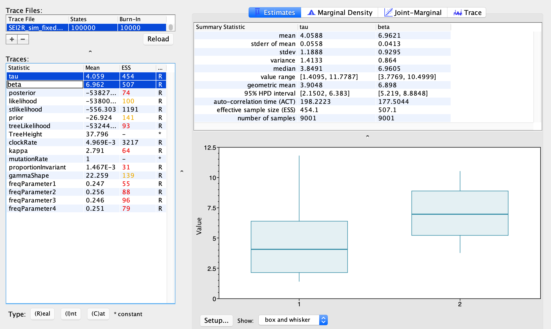
We can look at the posterior distributions inferred for our epidemiological parameters \(\beta\) and \(\tau\). The true transmission rate was 5.0 in our simulations, and the transmission rate from high risk individuals was 5X higher than low risk individuals, so the true value of \(\tau\) is also 5.0. We can compare these true values to our posterior estimates. Using my simulated data, the median posterior estimate of \(\tau\) is a little low and the median posterior estimate for \(\beta\) is a little high, but the true values are or nearly contained within the 95% credible intervals. Since these two parameters are highly correlated and its likely difficult to infer their precise values individually, I’m willing to accept that these are reasonably good estimates. Ideally we would simulate multiple data sets to test the overall accuracy and for any systematic biases in our estimates, but since we all simulated our own data set we already have some degree of replication. What do your parameter estimates look like?
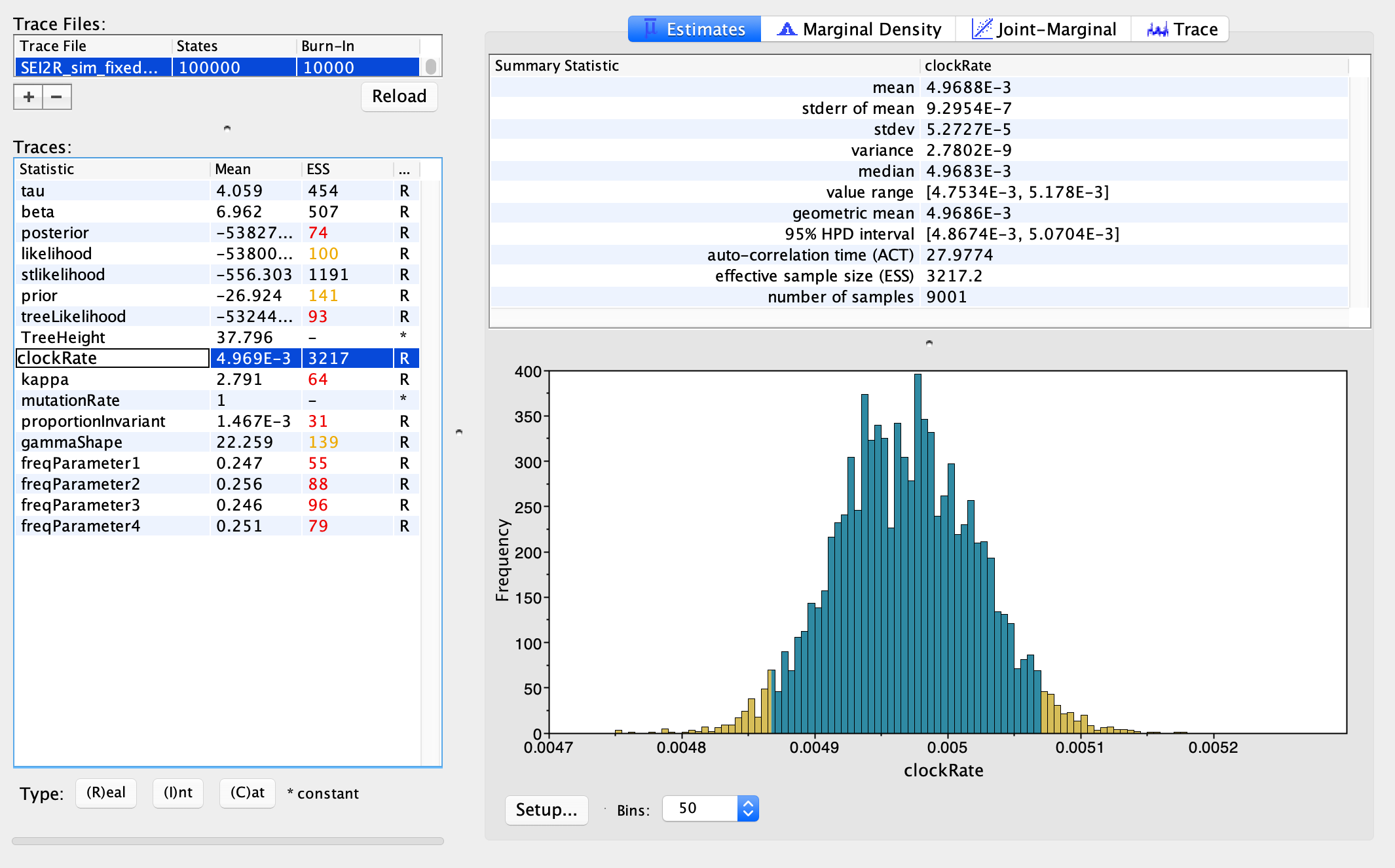
As another sanity check, we can also make sure that we can accurately estimate the parameters of the evolutionary model back from the sequence data. For example, the molecular clock rate we used to simulate the sequences was 5.0 x 10^-3, and the posterior median estimate is 4.97 x 10^-3 from my simulated sequence. So pretty darn good!
Applying the SEI2R model to SARS-CoV-2 genomic data
Now that we are reasonably confident that the SEI2R model is working correctly, let’s apply it to some empirical SARS-CoV-2 genomic data. I downloaded 166 SARS-CoV-2 full length genomes from the GISAID database. All of these samples were isolated between late February and mid-March of 2020 from patients in Washington state, one of the first epicenters of the US epidemic.
To save you time, I already aligned these sequences and put the resulting alignment and sampling times in a modified version of the XML template we used above. I also added an input starting tree that I reconstructed in BEAST. You can download the XML file with the SARS-CoV-2 data here.
The SEI2R model is exactly the same as before but we will walk through some of the changes I made to the XML file. First, I made some dramatic changes to the epidemiological model parameters in the rates element:
<rates spec="ModelParameters" id='rates'>

  <!-- Incubation period is about 5.5 days so eta should be (1/5.5)*365 = 66.36 per yr -->

  <!-- To follow 80/20 rule: we'll assume eta_l = eta * 0.8 = 53 per yr -->
  <param spec='ParamValue' names='eta_l' values='53.0'/>

  <!-- To follow 80/20 rule: we'll assume eta_h = eta * 0.2 = 13.27 per yr -->
  <param spec='ParamValue' names='eta_h' values='12.27'/>

  <!-- Infectious period is assumed to be 12 days so gamma should be (1/12)*365 = 30.45 per yr-->
  <param spec='ParamValue' names='gamma' values='30.45'/>

  <param spec='ParamValue' names='beta' values='@beta'/>
  <param spec='ParamValue' names='tau' values='@tau'/>
</rates>
The sampling times are given in years rather than in days as they were before, so all per day rates have been multiplied by 365 to get rates per year. I’ve also changed some of the model parameters to be more suitable for Covid-19. I’ve changed the incubation rate \(\eta\) to reflect the mean incubation period for Covid-19, which has been estimated to be 5.5 days (Lauer et al., 2020).
All sampled individuals are assumed to be in the low risk group. We do not know what fraction of infections are high or low risk, or even if there is considerable transmission heterogeneity among individuals, but we will continue to assume the 80-20 rule and have 20% of exposed individuals incubate into the high risk group. We will try to infer whether there actually is significant differences in transmission rates between hosts be estimating \(\tau\) from the phylogeny.
Finally we will assume that the mean infectious period is about 12 days, so the recovery rate \(\gamma\) is now \((1/12) \times 365 = 30.45\) per year.
In the trajparams element we need to set the starting time t0 as a date in years. I’ve set this to 2019.80, immediately before the estimated root time of the tree. This is less than ideal because we know the epidemic in Washington state did not start until much later in February, but we need to know the early epidemic trajectory in order to be able to compute the likelihood of the phylogeny since there are lineages in the tree that predate the WA state epidemic. A better model would include viral imports from external sources, but I will leave that for the ambitious among you to implement!
<trajparams id='initValues' spec='TrajectoryParameters' method="classicrk"
            integrationSteps="400" t0="2019.80">
    <initialValue spec="ParamValue" names='S' values='9999.0'  />
    <initialValue spec="ParamValue" names='E' values='0.0'  />
    <initialValue spec="ParamValue" names='Il' values='0.0'  />
    <initialValue spec="ParamValue" names='Ih' values='@initI0'/>
    <initialValue spec="ParamValue" names='R' values='0.0'  />
</trajparams>
Next, let’s look at the prior on the molecular clock rate. All of our samples were collected over a period of less than a month, so there is probably not enough temporal signal in the sequence data to be able to infer the clock rate without prior information. Looking at clock rate analysis on NextStrain, the current best estimate is about 25 substitutions per genome per year, so about 8 x 10^-4 substitutions per site per year given that the SARS-CoV-2 genome is about 30kb. So I have set a very informative LogNormal prior on the clock rate with mean equal to 8 x 10^-4 and and a standard deviation of 0.2 which places about 95% of the prior probability density on values between 6 x 10^-4 and 1.0 x 10^-3:
<prior id="ClockPrior" name="distribution" x="@clockRate">
    <!-- Prior mean is 8.0 x 10^-4 with 95% CI 6 - 10 x 10^-4-->
    <LogNormal id="LogNormalDistributionModel.1" meanInRealSpace="true" name="distr">
        <parameter id="parameter.hyperLogNormalDistributionModel-M-ClockPrior" estimate="false" name="M">0.0008</parameter>
        <parameter id="RealParameter.4" estimate="false" lower="0.0" name="S" upper="5.0">0.2</parameter>
    </LogNormal>
</prior>
We will again estimate the epidemiological and evolutionary model parameters but fix the phylogenetic tree for now. However, if you would like to go back and perform the analysis while inferring the tree, all you need to do is uncomment the following tree operators by deleting the <!-- and –--> surrounding the operators. As it stands now, having these operators commented out means that BEAST will never propose new trees during the MCMC.
<!-- Operators on tree -->

<!--
    <operator id="strictClockUpDownOperator" spec="UpDownOperator" scaleFactor="0.75" weight="3.0">
        <up idref="clockRate"/>
        <down idref="tree"/>
    </operator>

    <operator id="TreeScaler" spec="ScaleOperator" scaleFactor="0.5" tree="@tree" weight="3.0"/>

    <operator id="TreeRootScaler" spec="ScaleOperator" rootOnly="true" scaleFactor="0.5" tree="@tree" weight="3.0"/>

    <operator id="UniformOperator" spec="Uniform" tree="@tree" weight="30.0"/>

    <operator id="SubtreeSlide" spec="SubtreeSlide" tree="@tree" weight="15.0"/>

    <operator id="Narrow" spec="Exchange" tree="@tree" weight="15.0"/>

    <operator id="Wide" spec="Exchange" isNarrow="false" tree="@tree" weight="3.0"/>

    <operator id="WilsonBalding" spec="WilsonBalding" tree="@tree" weight="3.0"/>

  -->
You can now run the analysis in BEAST using the WA_cov2020_SEI2R_fixedTree.xml file.
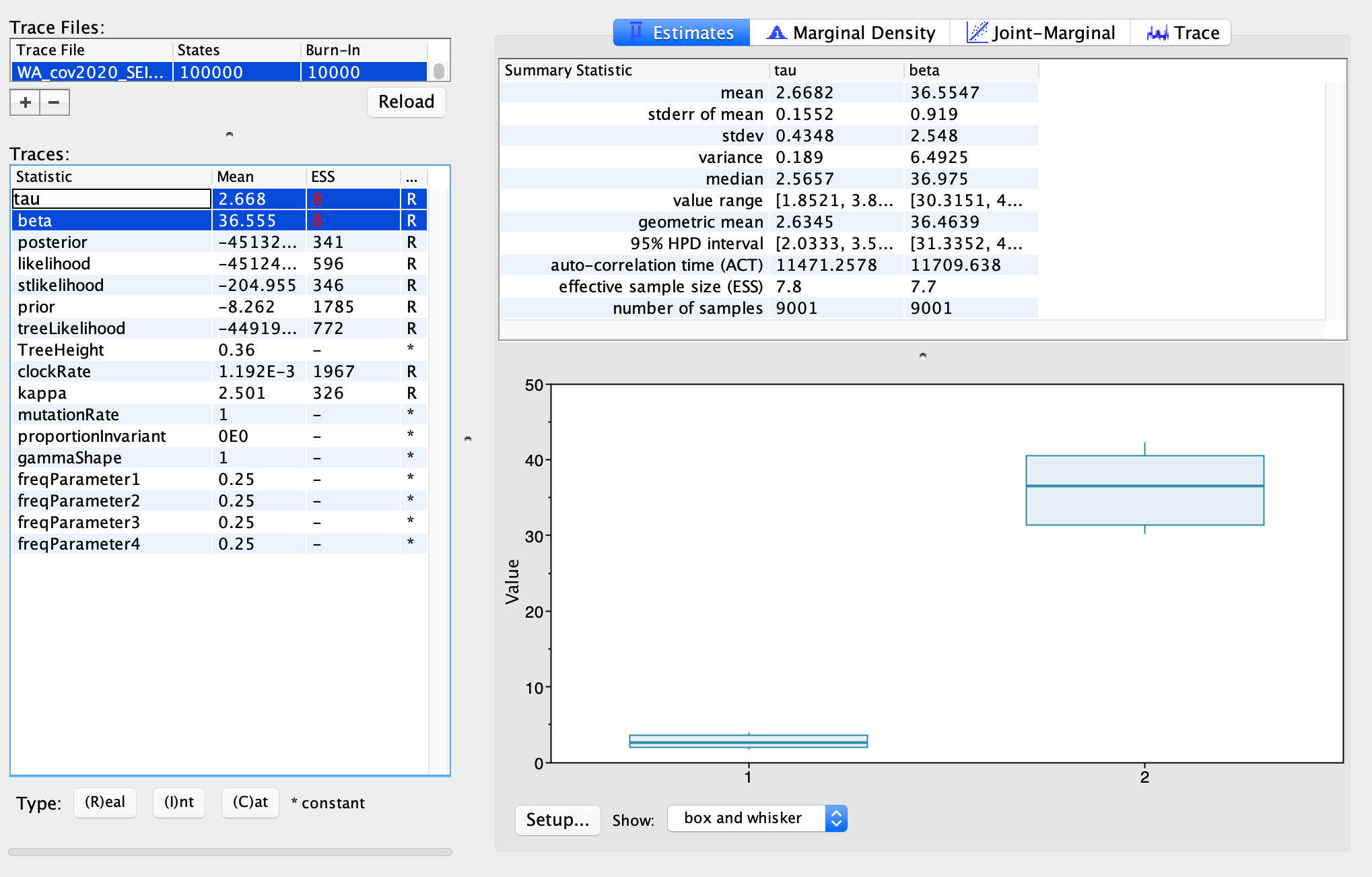
After the MCMC finishes running in BEAST, open the .log file in Tracer to explore the posterior estimates. With only 100,000 iterations, I was not able to get good MCMC mixing, which would explain the very low effective sample sizes (ESS) for some of the parameters. So ideally we would run the MCMC for much longer.
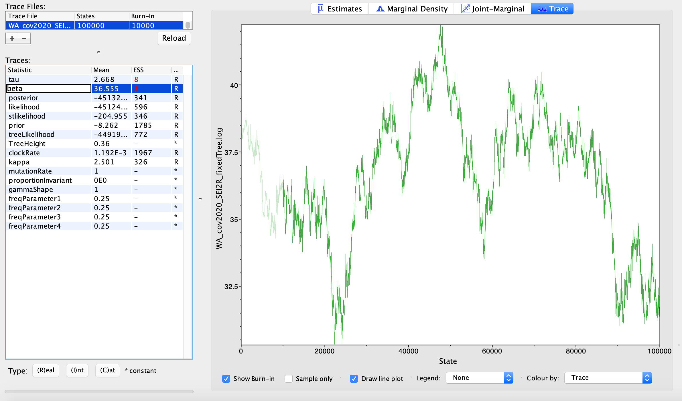
Nevertheless, we can cautiously interpret some of our preliminary estimates. The median posterior estimate for the transmission rate \(\beta\) for low-risk hosts is 36.975. We assumed a mean recovery/removal rate of 30.45, so if we only consider low-risk individuals \(R_{0} = \frac{\beta}{\gamma} = 1.21\). But our median estimate of \(\tau\) shows that high-risk individuals are about 2.5 X more infectious. In order to get an estimate of the overall \(R_{0}\) we need to take into account the contribution of both low and high risk individuals. Using a next-generation approach, I calculated that the overall \(R_{0}\) is about 1.57.
Taken together, these estimates suggest that the transmission rate in the general population is fairly low but high-risk individuals considerably increase overall transmission. The unsatisfying thing here is that we don’t know what makes high-risk individuals high risk because we simply assumed that 20% of exposed hosts become high-risk. It may be that the high-risk group represents individuals with greater number of social contacts. These high-risk individuals could also represent asymptomatic individuals who do not realize they are infected and so do not quarantine themselves.
Question for thought: We estimated that high-risk individuals are 2.5X more infectious than low-risk individuals even though we assumed all sampled individuals are low risk. What about the SARS-CoV-2 phylogeny do you think is informing our estimates about differences in transmission rates between risk groups?
References and Acknowledgments
Thank you to Igor Siveroni for help troubleshooting the XML file for the SEIR model.