Discrete trait phylogeography
What you will need:
-BEAST v.2.5.0 or greater
-Tracer v1.7.0 or greater
-FigTree
For postprocessing (optional):
-Spread
-Google Earth Pro
Exploring the origins of Phytophthora infestans
In this tutorial, we will use discrete trait phylogeographic methods to explore the origins Phytophthora infestans, the pathogen that causes potato late blight and started the Irish potato famine. Two origins have been postulated for the origins of P. infestans. Gómez-Alpizar et al. (2007) concluded that P. infestans likely arose in the Andean region of South America based on a coalescent analysis of mitochondrial and nuclear genes and the fact that P. infestans infects many different Solanaum hosts native to the Andes. On the other hand, Goss et al. (2014) concluded that P. infestans likely arose in the Toluca Valley of Central Mexico. They showed that the Toluca Valley contains diverse, sexual populations of P. infestans and their phylogeographic analysis showed all modern lineages sharing a common ancestor in Central Mexico.
We will reanalyze the dataset of Goss et al. (2014) using a discrete trait phylogeographic methods to see how they arrived at this conclusion. The data were kindly provided by Niklaus Grunwald and Javier Tabima at Oregon State.
Phylogeography in BEAST 2
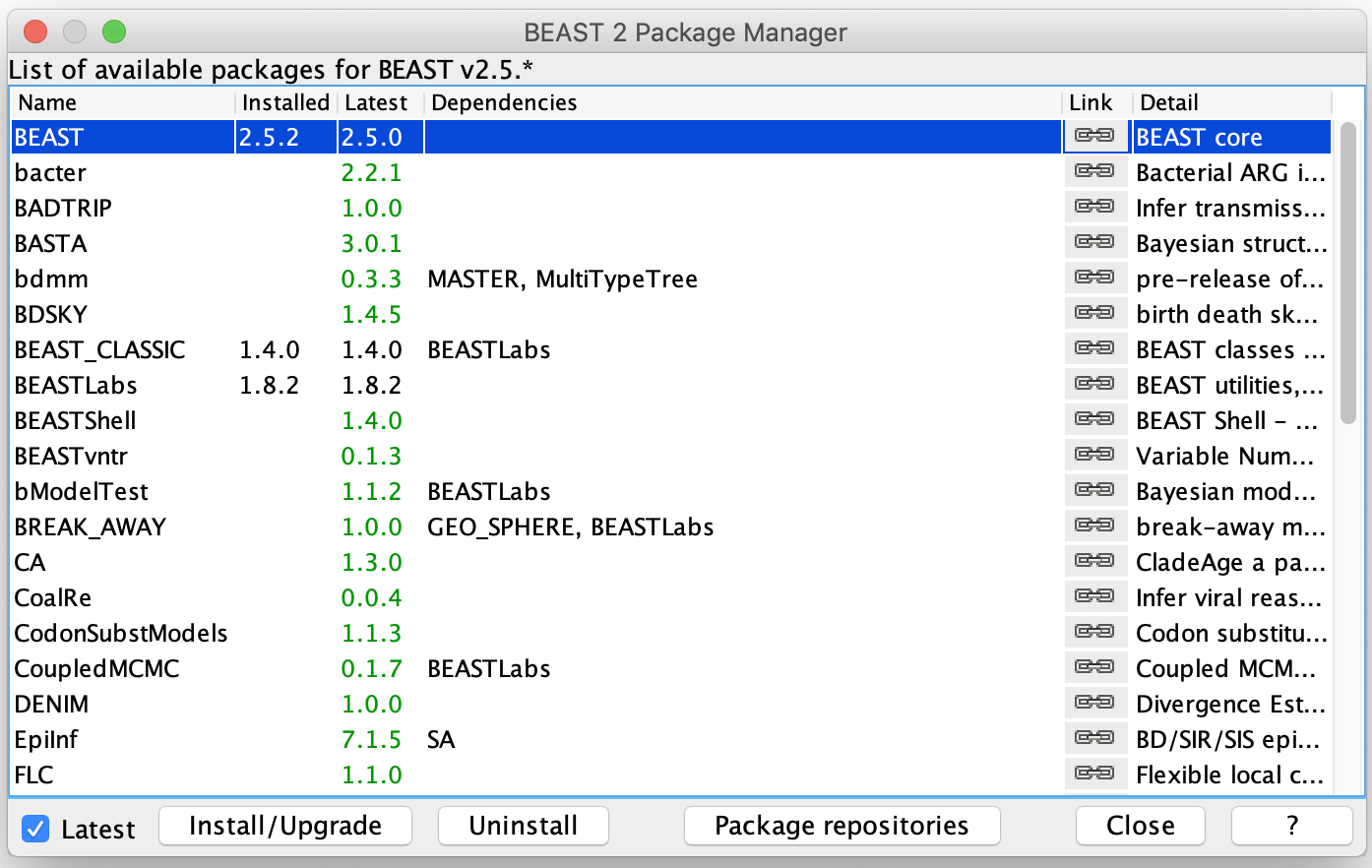
The discrete trait phylogeographic models we will use were originally implemented in BEAST version 1, but can be accessed in BEAST 2 through the BEASTlabs and BEAST-CLASSIC add-on packages.
To install these packages, open BEAUTi and select File → Manage Packages. In the dialog box that pops up, first select BEASTlabs and then click the Install button. Then install the BEAST-CLASSIC package. Once both packages are installed, restart BEAUTi so that the changes take affect in BEAUTi.
The seqeunce data
Goss et al. (2014) analyzed a diverse set of P. infestans isolates sampled from locations around the world. Four nuclear genes were sequenced from these isolates and then combined into a single multi-locus phylogeographic analysis. To speed up our BEAST runs, we will only analyze a single nuclear gene at a time. We can then see if the different genes all support a common geographic origin for P. infestans.
Choose one of the nuclear genes to analyze and download the aligned sequences for that loci using one of the links below:
Alignements:
Note
The aligned FASTA files contain the sampling location of each sequence in the headers. In the original analysis, Goss et al. included sequences from 13 discrete states (i.e. countries). While it is computationally feasible to have this many locations, this means that 13 x 13 = 169 migration rate parameters need to be estimated, one between each pair of locations. To simplify things, I grouped all countries in continental Europe (Estonia, Hungary, Netherlands, Poland, Sweden) into one location: ‘EU’. Grouping or binning nearby locations is a commonly employed strategy in phylogeography. Furthermore, I removed samples from two countries (Vietnam and South Africa) for which there were only a few samples. After grouping and cutting, there are seven discrete locations in our analyses.
Setting up the analysis
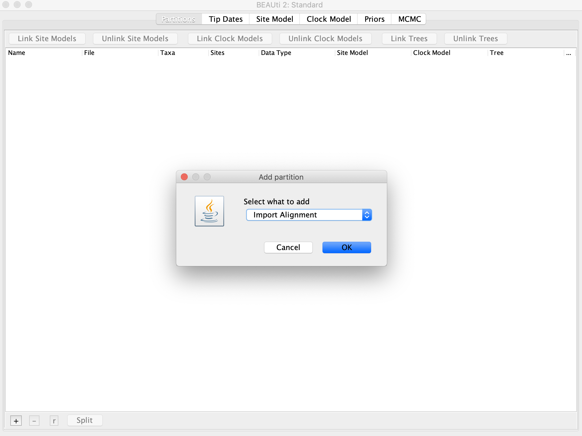
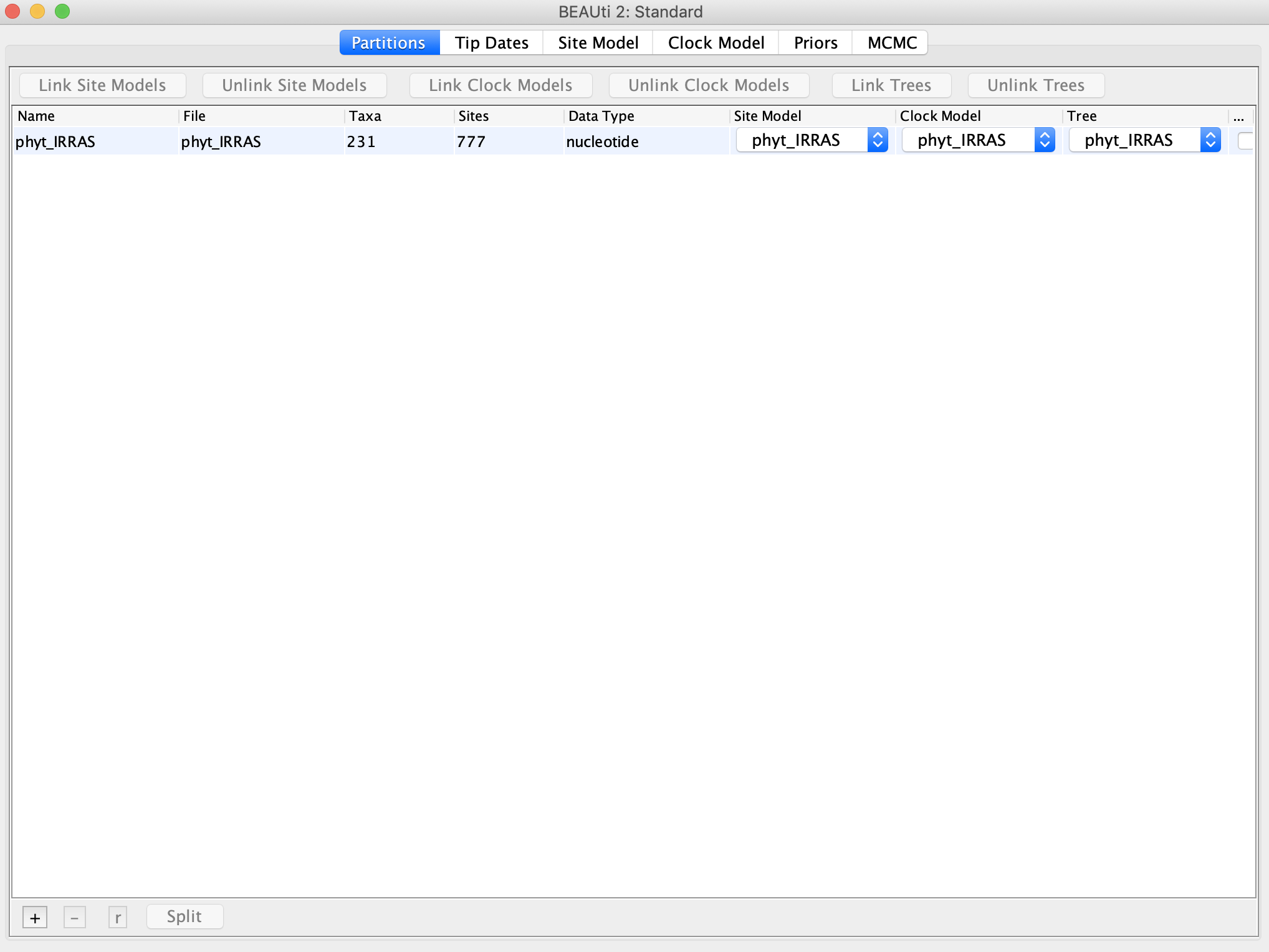
Reopen BEAUTi and click the + button on bottom left of the Partitions tab. Select Import Alignment, click OK, and then import the appropriate alignment file (e.g. phyt_IRRAS_labeledByCountry.fasta) for the nuclear gene you chose.
We will assume all samples are contemporaneous (i.e. sampled at the present) so we do not need to add anything in the Tip Dates panel.
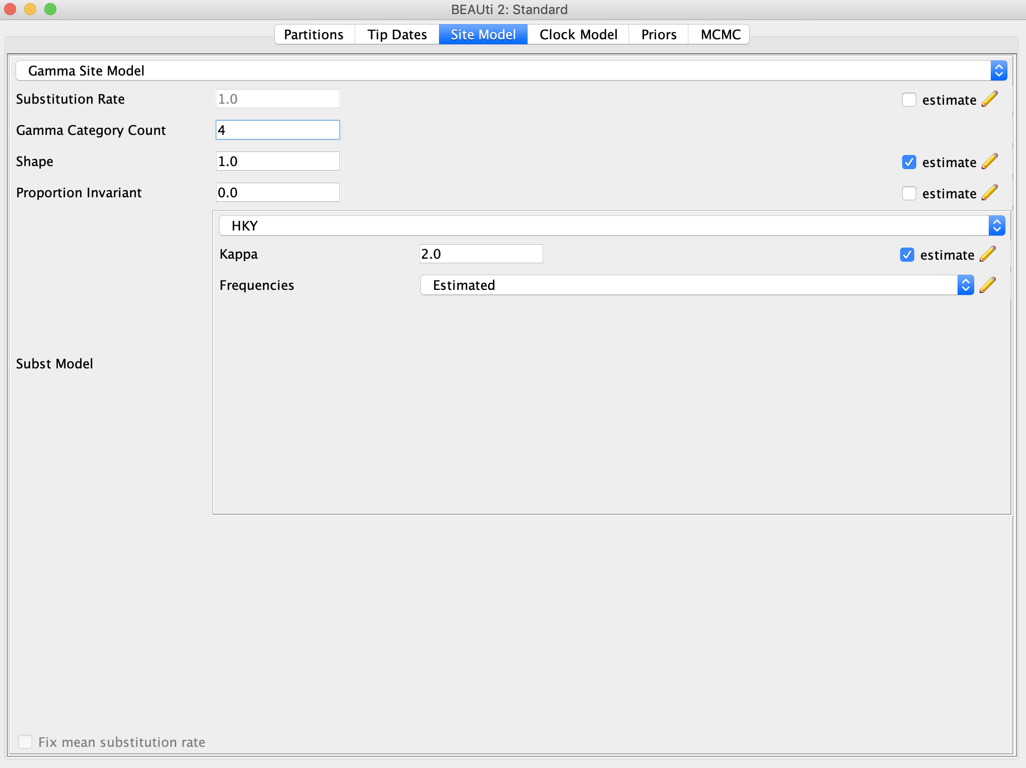
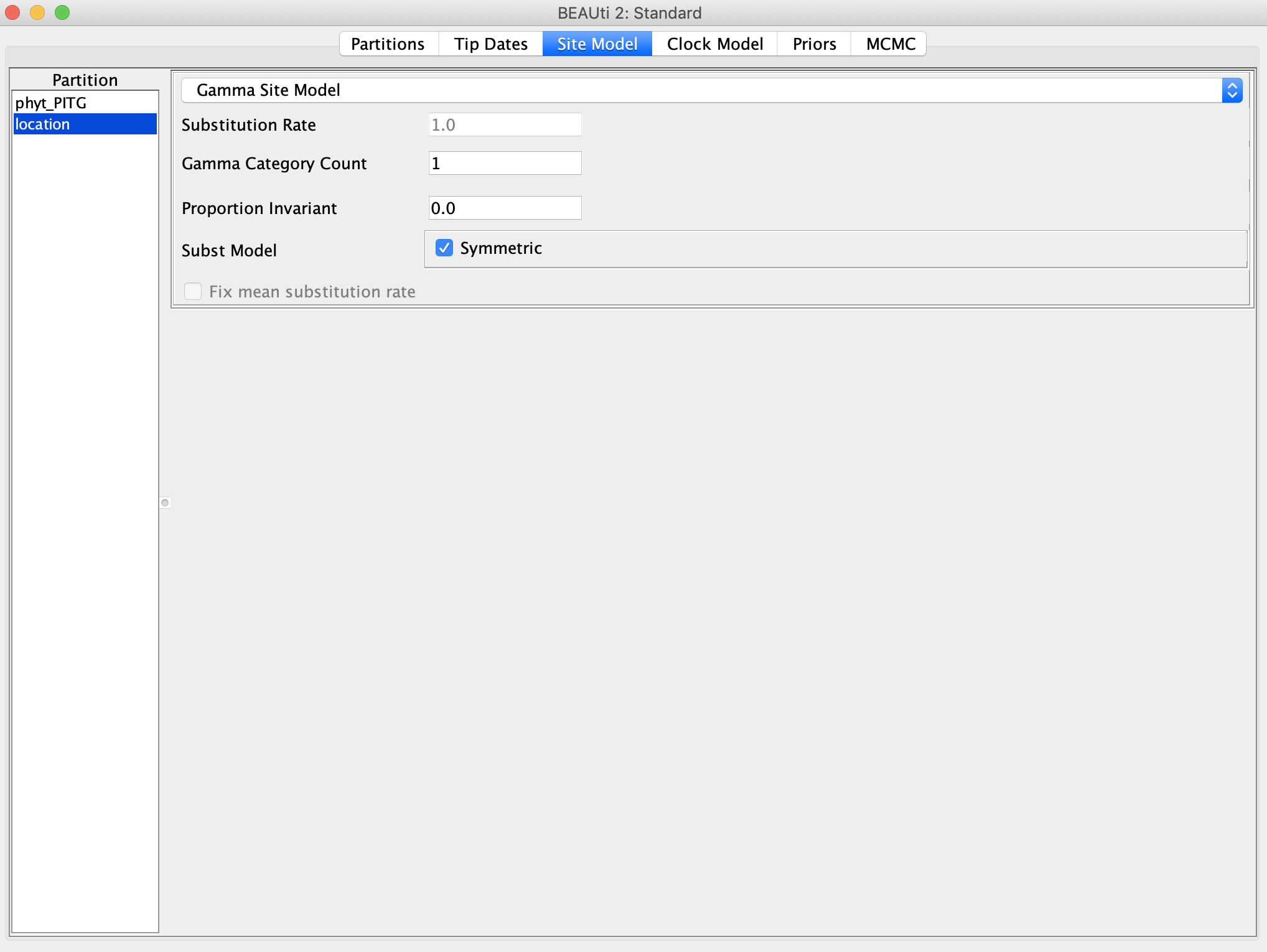
In the Site Model panel, we will use a gamma site model with four rate categories, so enter ‘4’ next to Gamma Category Count. A HKY substitution model should be sufficient for this data. The Site Model panel should now look like this:
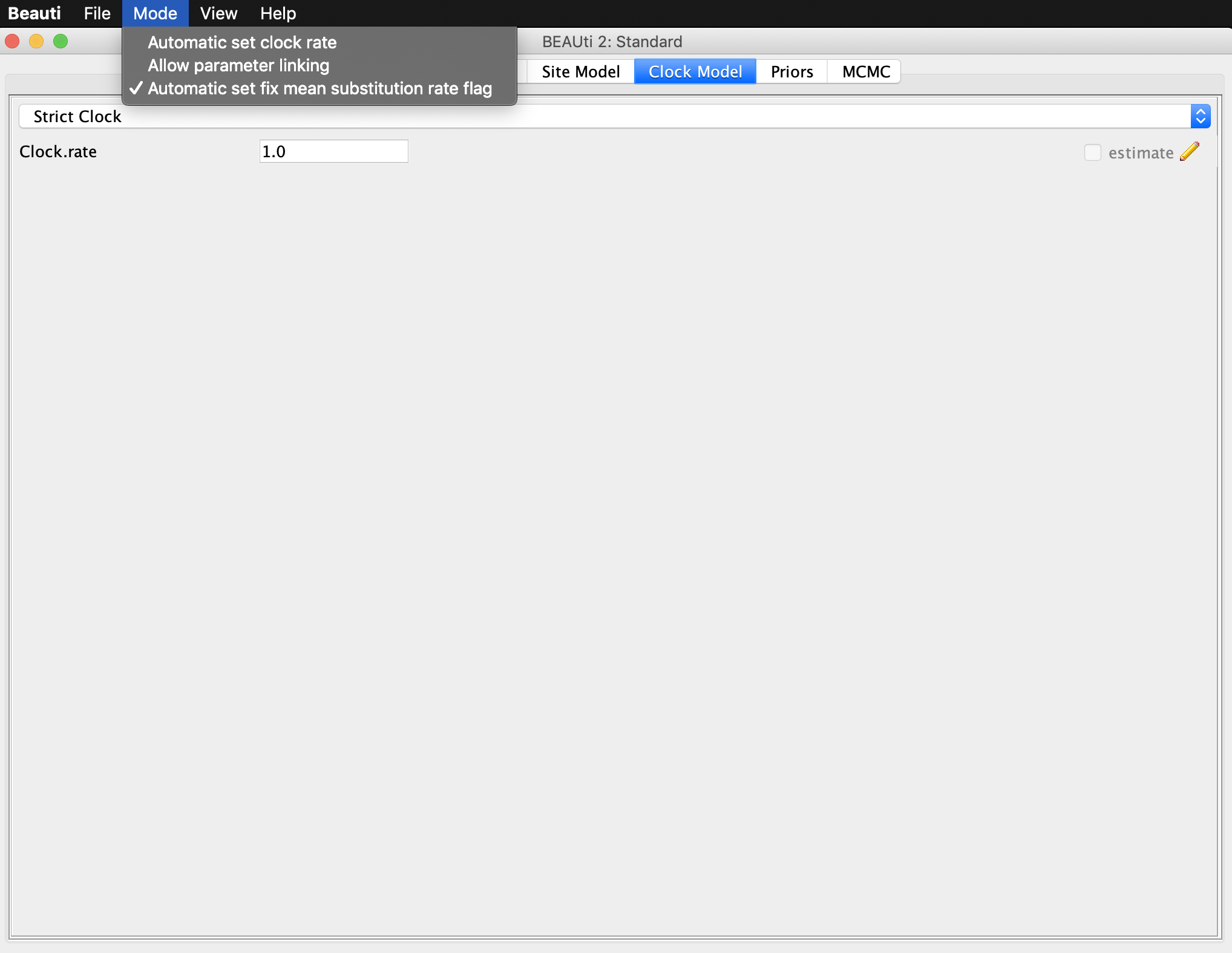
Now go to the Clock Model panel. We we will use a strict clock model but we do not have a way of calibrating the clock rate, so we can guess something reasonable for eukaryotic nuclear genes so that we are working on a reasonable time scale, I chose 0.00001. We should therefore not place too much weight on our estimated branch lengths and node heights, but we can still reconstruct the ancestral location of lineages through time. We therefore want to fix our clock rate at this value, but BEAST likes to enforce that we either estimate the clock rate or the overall substitution rate. To prevent this from happening click Mode and then unselect Automatic set clock rate.
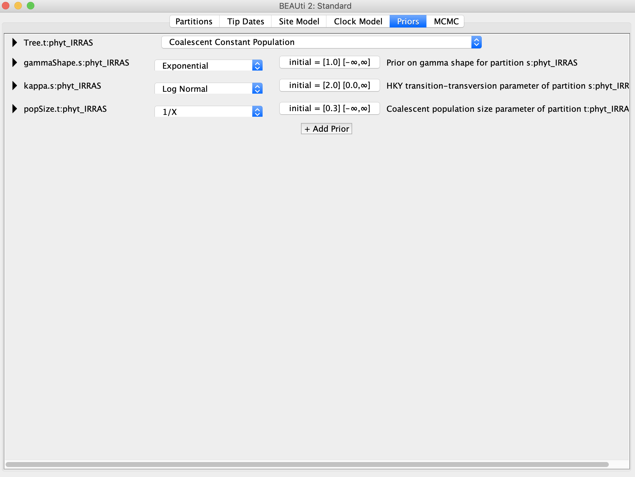
In the Priors panel, we will use a Coalescent Constant Population tree prior. The other priors can be left at their default settings.
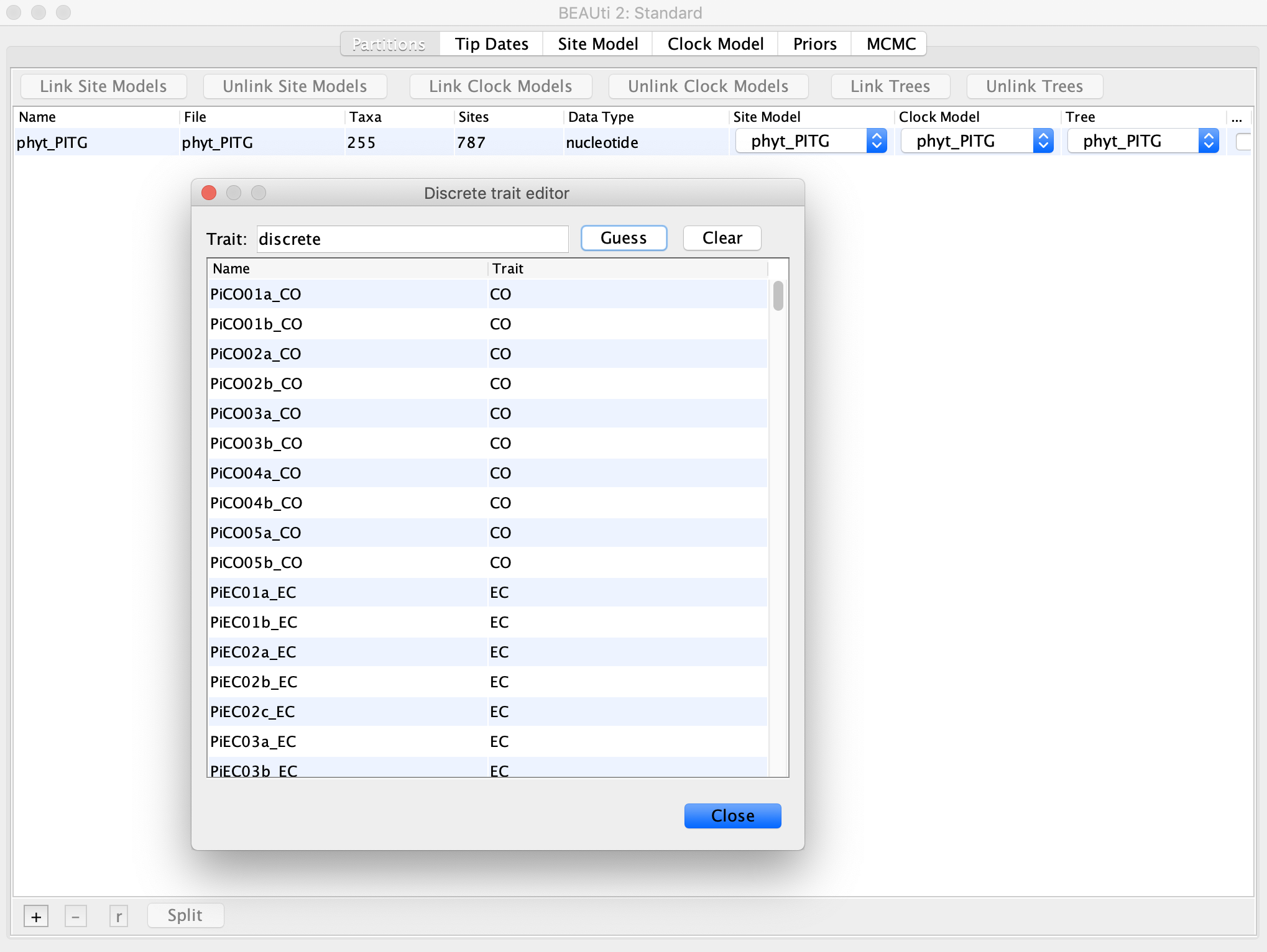
Now we want to add the sampling location of each tip, which will be the discrete trait in our analysis. BEAST treats this trait data very similar to sequence data, which makes sense because in essence we are adding another partition to the sequence alignment with one more “site” representing the sampling locations. Go back to the Partitions panel and click the + button again on bottom left. This time select Add Discrete Trait. You can now give the trait a name such as location, and then associate/link the tree for the discrete trait with the name of the tree from the sequence alignment.
In the new window that pops up we will now associate each taxon name with its sampling location. Lucky for us, the sampling locations are already contained within the names. Click Guess and then select use everything after first underscore. The traits should now be automatically populated with the correct sampling locations, but make sure that the locations correspond to the correct sampling locations in the taxon names!
Go to the Site Model panel a second time and select location from the different partitions on the left. The site model here is analagous to the substitution model we used for the sequence data, except now the substitution rate matrix gives the relative migration rate between each location. We will use the default Symmetric model.
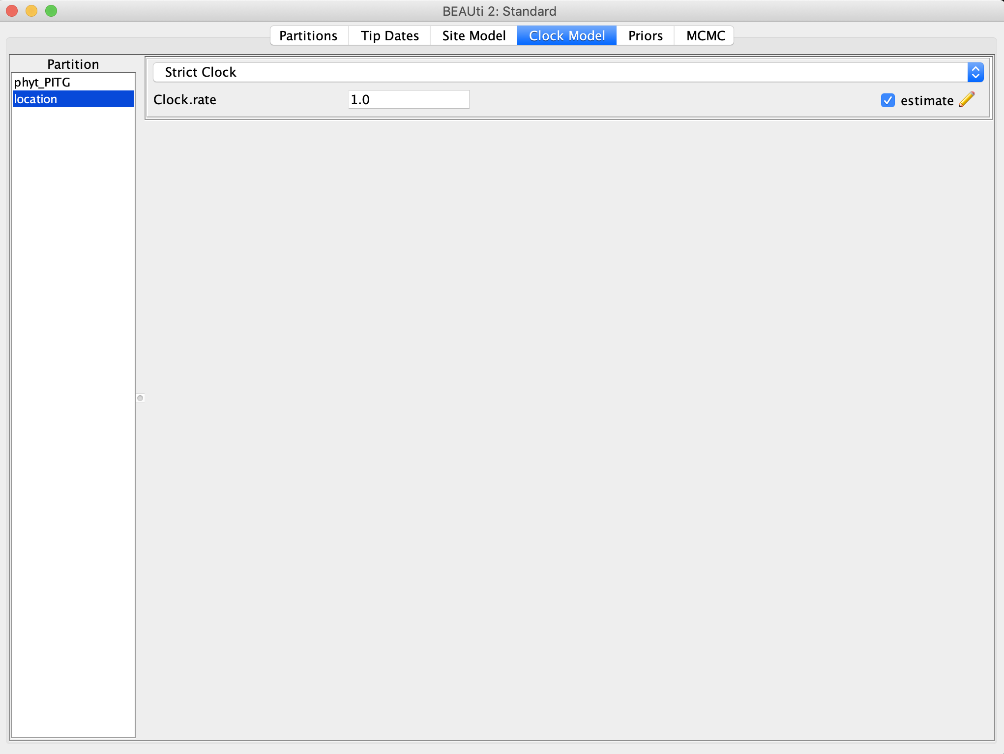
Go to the Clock Model panel and select the location partition. We will use a strict clock model again, but now this clock rate controls the absolute rate at which lineages transition between different locations. Make sure the estimate box is checked on the right.
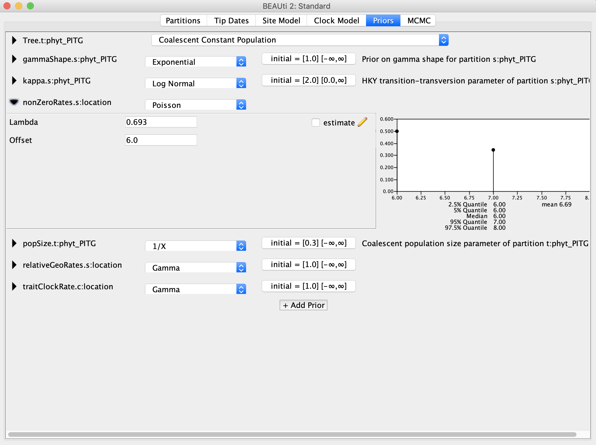
Now we need to set up some priors for our discrete trait in the Priors panel. For the nonZeroRates we can continue to use a Poisson prior with lambda = 0.693. This prior is used for Bayesian Stochastic Search Variable Selection. Lambda is the prior probability that a given migration rate between two locations will be nonzero. We will use BSSVS to estimate which migration rates are nonzero and which can be constrained to zero, resulting in a lower dimensional model with fewer parameters to estimate.
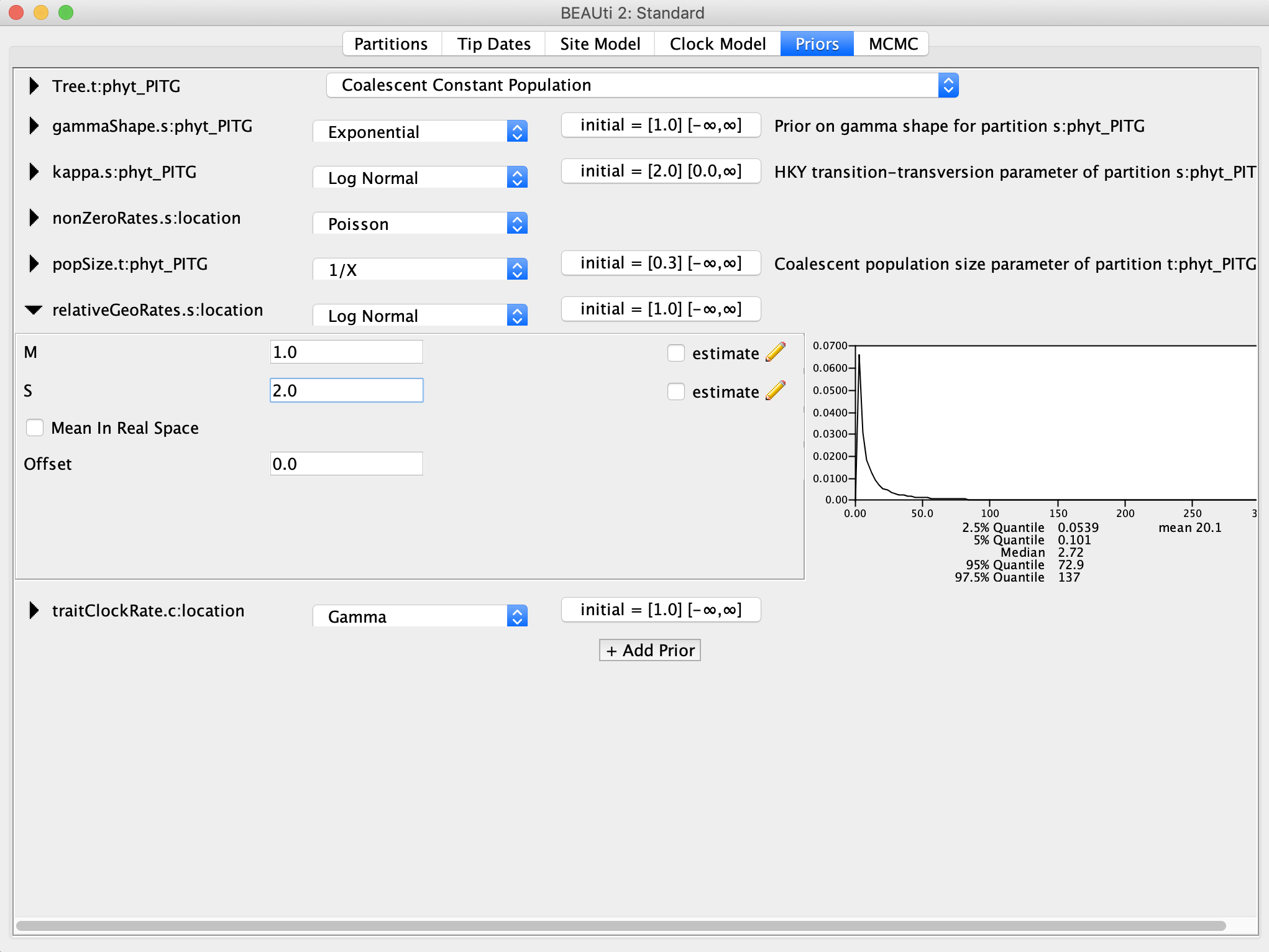
For the relativeGeoRates and traitClockRate, I recommend Log Normal priors. When in doubt, a Log Normal prior is good choice for a prior for rate parameters because the distribution is constrained to positive values, which is good because we cannot have negative rates. We can then center the prior density around our best guess for the value by setting the mean, and how concentrated the prior density is around the mean using the variance or standard deviation. For this analysis, I set the mean M equal to 1.0 and the standard deviation S to 2.0, so that we have a fairly uninformative prior with a long right tail.
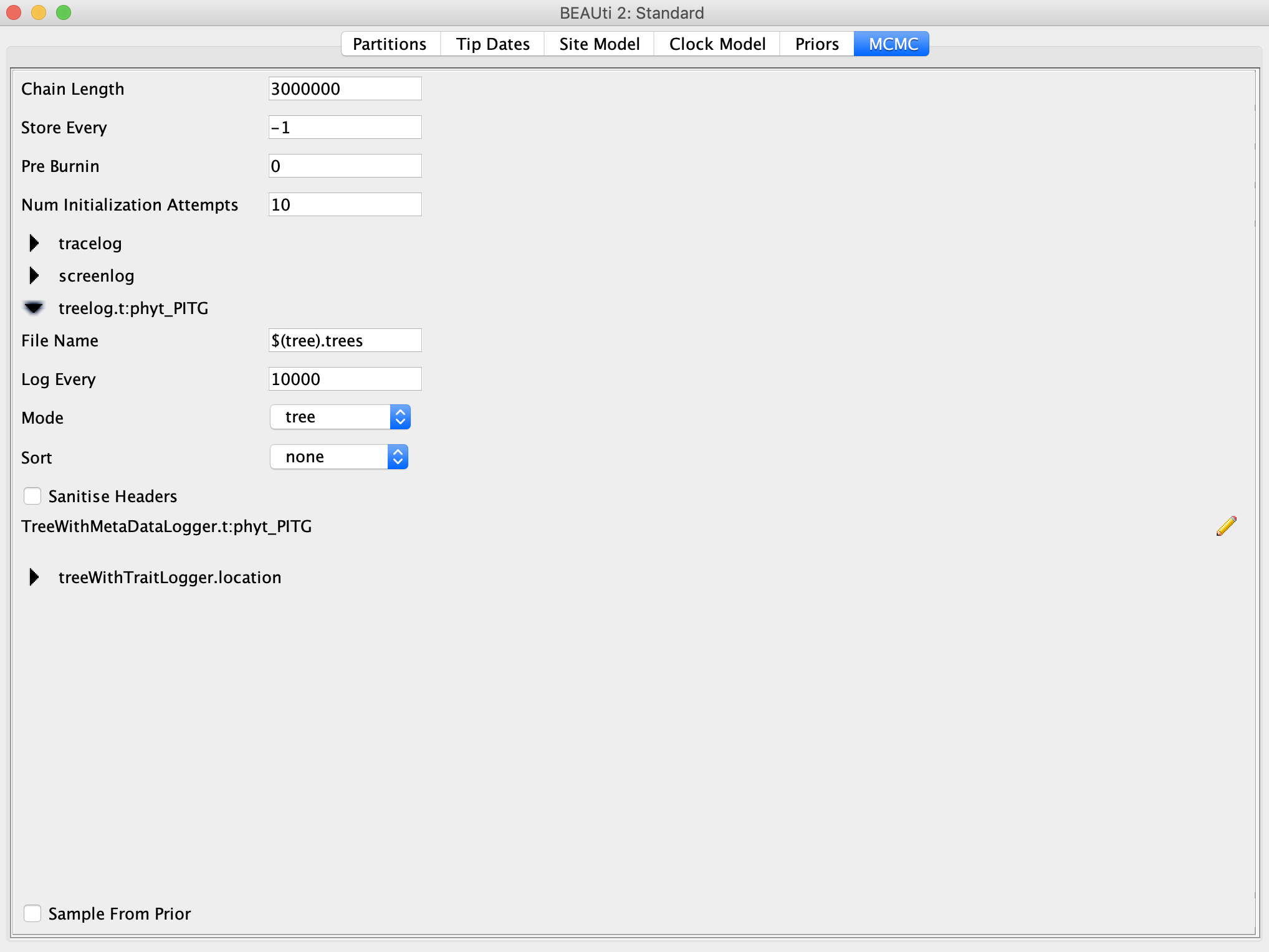
Go to the MCMC panel and set the Chain Length to 3 million. For a definitive (i.e. publishable) analysis, we would probably want to run the MCMC for much longer, but we don’t have all day. I would also recommend going under the treelog drop down menu and setting Log Every to 10,000, otherwise BEAST will write out the tree every 1,000 iterations and the tree file will become huge.
Finally, select File → Save As to generate the XML file to input into BEAST. We’ve now set up our entire analysis!
Running BEAST and analyzing the results
Open BEAST and choose the XML file we just generated and hit Run.
Once BEAST is finished running, open Tracer and then import the .log file from your BEAST run. We can use Tracer to explore the posterior estimates of some key parameters like the absolute migration rate (traitClockRate) and the relative migration rates between locations (relGeoRates).
If for some reason you were not able to get the analysis set up in BEAUTi or run it in BEAST, you can download example log and tree files for the analysis of the PITG gene I ran.
Visualizing the phylogeographic reconstructions
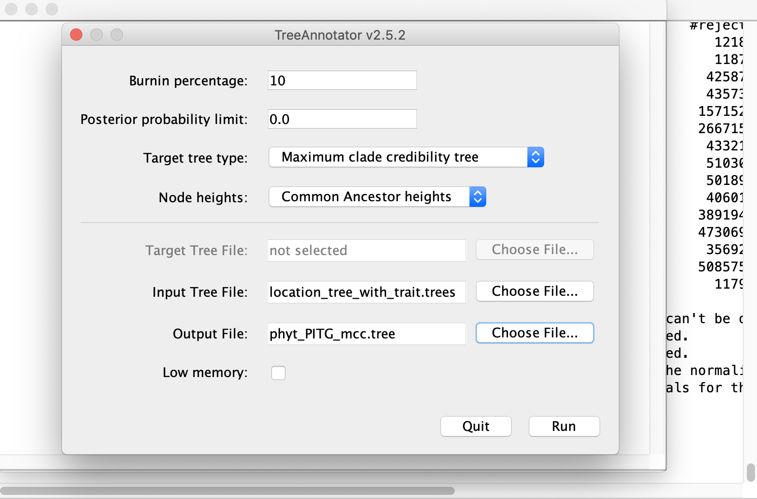
We can summarize the posterior distribution of trees and reconstructed ancestral states as a single concensus (MCC) tree in TreeAnnotator. Open TreeAnnotator and for the Input Tree File select the location_tree_with_trait.trees file that BEAST generated. For the Burnin percentage, we can use 10%. Make sure that Maximum clade credibility tree is selected for Target tree type. Select an Output File name for the MCC tree such as phyt_PITG_mcc.tre. Now press Run.
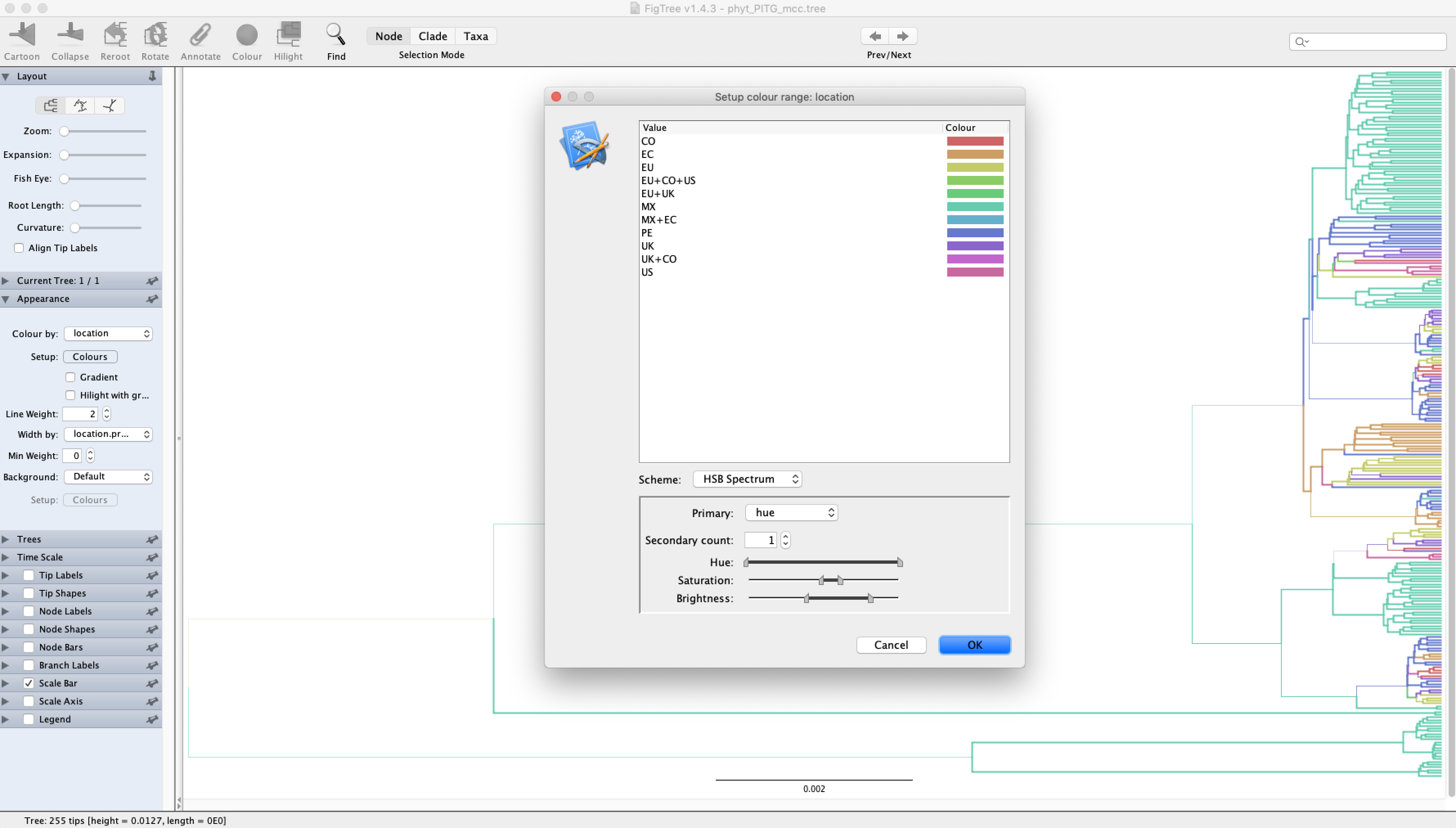
Open the consensus MCC tree you just generated in FigTree. Select Appearance, and then choose location under Colour by. The lineages in the tree will now be colored by their most probable ancestral location – the state with the highest posterior probability. You may want to increase the Line Width to make this easier to see. You can also have the branch widths reflect the posterior support or probability for the ancestral states by selecting location.prob under Width by.
Questions for discussion
The MCC tree shown above for my analysis of the PITG gene seems to support a rooting of P. infestans in Mexico. What does your analysis show?
- Do all the nuclear genes support a geographic origin in Mexico?
- How much confidence should we place in the ancestral state/location reconstructions?
- We only included samples from modern lineages. Do you think our results apply to the origin of the famine lineage that spread to Europe in the 19th century?
- The dataset contained a large number of samples from Mexico. Do you think we would obtain the same results if we sampled less from Mexico?
Visualizing geographic spread
Download Spread if you haven’t already. Unfortunately, the Mac version does not seem to work on newer versions of Mac OS, but you can download the .jar file provided for Windows/Linux users using the link above.
It may then be possible to launch the jar file can from the command line:
java -jar SPREAD\ v1.0.7.jar
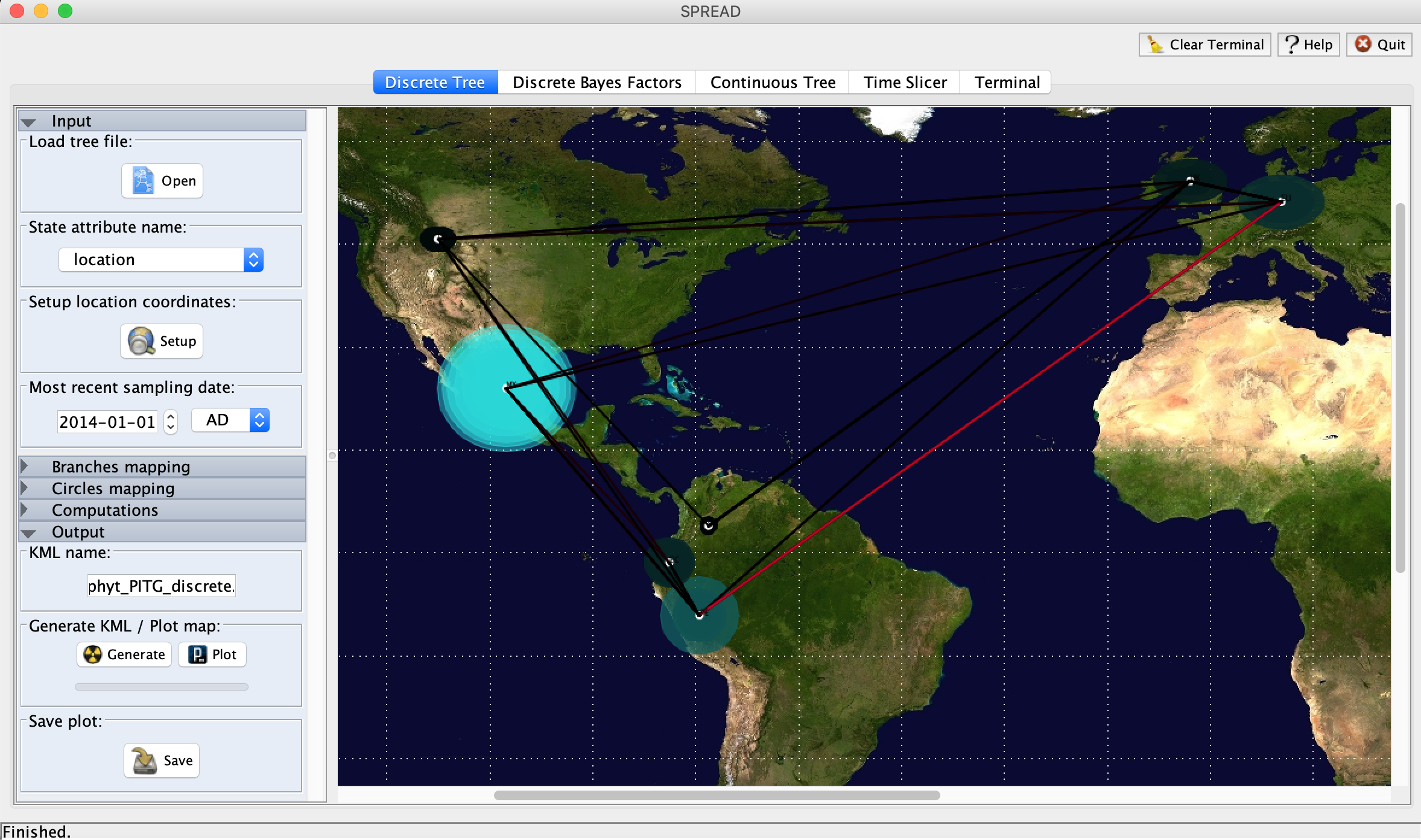
In Spread, select Open → Load tree file and then choose the consensus MCC tree file you created in TreeAnnotator. Under State attribute name select location.
If you click the Set-up button, you can manually edit the latitude and longitude coordinates of each discrete sampling location. I used the coordinates of the centroid of each country available here.
| Location | Code | Latitude | Longitude |
|---|---|---|---|
| Europe | EU | 51.1069 | 10.385 |
| Peru | PE | -9.152 | -74.382 |
| United Kingdom | UK | 54.123 | -2.865 |
| Mexico | MX | 23.947 | -102.523 |
| Columbia | C0 | 3.913 | -73.081 |
| Ecuador | EC | -1.423 | -78.752 |
| United States | US | 45.679 | -112.461 |
Note: If you need to find the geographic coordinates of more specific locations, you can always use Google Earth. Pointing the mouse cursor at a specific location will provide the longitude and latitude.
Clicking Display will show the migration events in the MCC phylogeny mapped onto the world map. The diameter of the circles shows how many lineages in the tree reside in a particular location at a particular time. The branch lengths are colored by their time ordering from oldest to youngest. Click the output button to generate a KML file.
Finally, you can create a video animating the spread of lineages through time and space that can be viewed in Google Earth. Download Google Earth Pro and open the application. Click File → Open, select the KML file you just generated and then click Open. The animation should play automatically and you can rewind or advance through the animation using the cursor at the top of the window.
Other phylogeography tutorials
Phylogeographic methods and related visualization tools have developed incredibly rapidly in the past decade and this tutorial is already somewhat out-of-date relative to the cutting edge. So below I’ve provided links to other tutorials using newer software. However, these tutorials are based on BEAST version 1.
There is another great tutorial on discrete-trait phylogeography exploring the spread of bat rabies here. This tutorial is also really neat because it shows how to create web-based visualizations in D3 using SpreaD3, the successor to Spread, and how to identify predictors of migration rates using Generalized Linear Models.
There is also a very cool tutorial on tracking the spread of West Nile Virus through North America using continuous-trait phylogeographic models here.
Acknoweledgments
This tutorial was based on an earlier tutorial by Remco Bouckaert on discrete traits models in BEAST 2.