Wrangling sequences and trees
What you will need:
-RAxML-NG (Precompiled versions for Mac, Windows and Linux)
-AliView or another sequence alignment viewer
-FigTree
-TempEst
Optional:
-Python 3.6 or later
-Biopython
If you plan to do the optional tutorial on wrangling sequences in Python, I will assume you have at least Python 3.6 installed on your computer. If not, the easiest way to get it is by installing the Anaconda distribution of Python. This comes with many standard scientific libraries like Numpy and Pandas, and makes installing additional packages like Biopython easy.
Windows users: This tutorial assumes you are using a Linux-style command line shell like bash. The easiest way to run a Linux Bash shell on Windows is probably the Windows Subsystem for Linux. Here’s some information on installing the WSL Bash shell.
Influenza A H3N2 in North Carolina
In this tutorial we will look at the phylogenetic history of human influenza viruses sampled in North Carolina over the past 10 years. These viruses are mostly influenza A subtype H3N2, which has been the dominate subtype of seasonal flu circulating in the human population since 1968. The data consist of full-length sequences of influenza’s hemagluttinin (HA) protein, which the virus uses to enter mammalian cells and is the major target of human antibodies against flu. All sequences were downloaded from the Influenza Research Database, taking all H3N2 subtype sequences collected in North Carolina from 2010 to 2019. We will use these sequences again in Week 4 to infer seasonal flu dynamics in NC from the flu phylogeny. A cleaned FASTA file containing the sequences is available here and on the GitHub repository for this tutorial.
Optional: Wrangling sequence data using Python
Analyzing sequence data inevitably involves some basic bioinformatics and data wrangling. Usually these are simple tasks like converting between file formats or renaming sequences, but if you have to do this manually it can become tedious and time consuming. Periodically through this class, I will show you how some data processing and analysis tasks can be easily performed in Python. If you’re not interested in coding or more comfortable using a different programming language, please skip ahead to the next section.
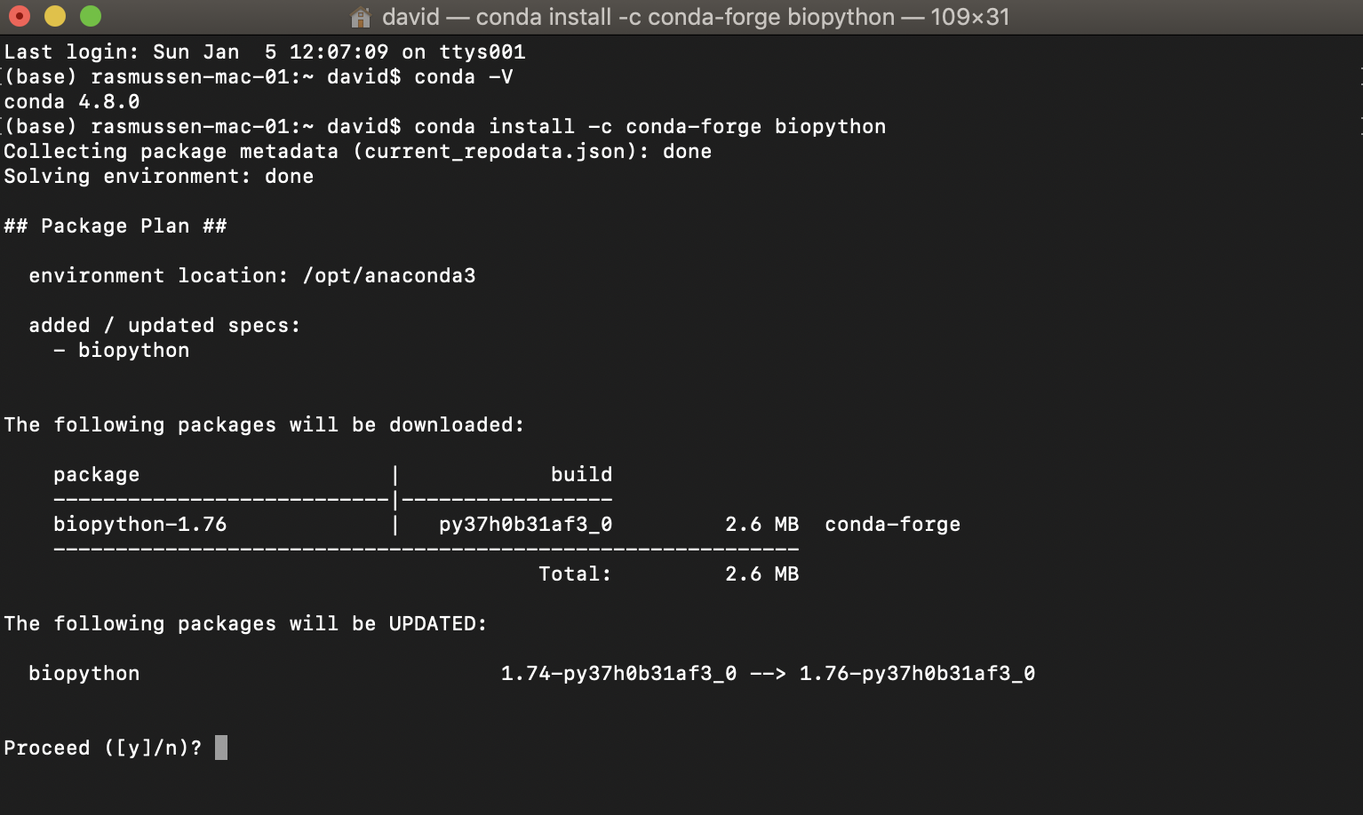
If you have installed the Anaconda distribution of Python, you can use the conda package manager to install Biopython. You can check if conda was correctly installed by typing conda -V at the command line (Terminal on a Mac). If so, install Biopython through conda by typing conda install -c conda-forge biopython. If you did not install Anaconda, directions for installing Biopython can be found here.
Next download the files get_genbank_records.py and influenzaA_H3N2_NC_2010-2019.tsv from the GitHub repository for this tutorial. Put both files in a folder or directory that is easy to access on your computer.
The python script get_genbank_records.py will download all sequences from NCBI GenBank for us. We just need to pass the Entrez interface in Biopython a comma-separated list of sequence accessions. We’ll use the Python library Pandas to quickly grab the list of sequence accessions from the .tsv file.
Note: We will run the actual script at the end of this section, you can just follow along with the code in the tutorial for now.
import pandas as pd
df = pd.read_csv('influenzaA_H3N2_NC_2010-2019.tsv','\t')
seq_list = df['Sequence Accession'] # get the seq accessions from the dataframe
seq_str = ",".join(seq_list) # a comma separated list of all sequence accessions
We can then download the actual sequence data from GenBank. Remember to change your email address in the get_genbank_records.py script so we tell NCBI who’s trying to access their servers.
from Bio import SeqIO
from Bio import Entrez
Entrez.email = "your_email@important_univ.edu" # Always tell NCBI who you are
handle = Entrez.efetch(db="nucleotide", id=seq_str, rettype="gb", retmode="text")
records = SeqIO.parse(handle, "gb")
At this point, we could simply write our new sequences to a fasta file using Biopython. But if we looked at the resulting FASTA file, we would notice that the sequence names (i.e. Headers) are not particularly succinct or nice looking:
>KC882595.1 Influenza A virus (A/North Carolina/01/2011(H3N2)) segment 4 hemagglutinin (HA) gene, complete cds
We will therefore clean these names up a bit and append sampling dates to the sequence names for easy access later. Since chances are high we’ll need to do this again, I’ve put this code in a separate function called rename_seqs.
def rename_seqs(records,df):

    "Iterate through list of records, renaming each as we go"
    new_records = []
    for record in records:
        accession = record.name # get accession number
        entry = df.index[df['Sequence Accession'] == accession].tolist() # get entry in df by accession number
        "Check to make sure entry exists and is unique"
        if len(entry) == 0:
            print("Entry not found for accession: " + accession)
        elif len(entry) > 1:
            print("More than one entry found for accession: " + accession)
        date = df.at[entry[0],'Collection Date'] # get date string
        record.id = accession + '_' + date # create new record id
        record.description = '' # set description blank
        new_records.append(record)

    return new_records
Once we have run rename_seqs, we can then write out our new sequence records as a fasta file using Biopyton’s SeqIO interface.
records = rename_seqs(records,df)
SeqIO.write(records, fasta_out, "fasta")
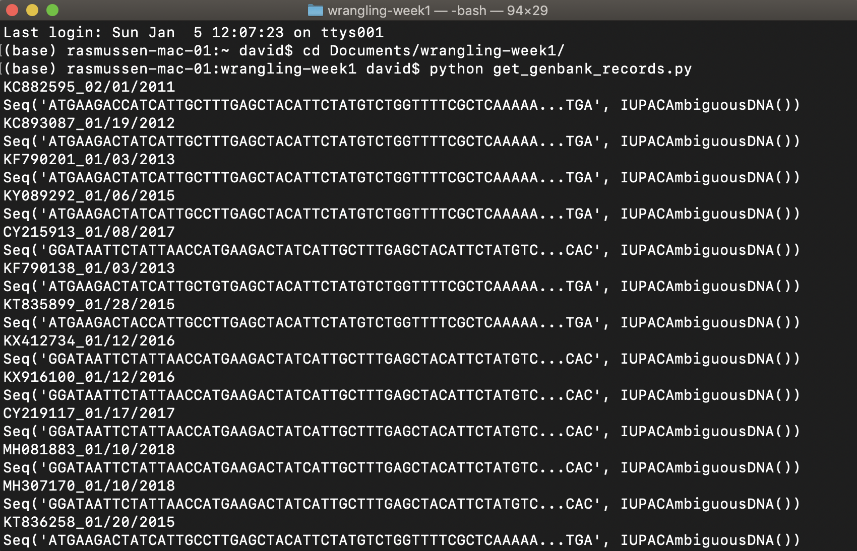
OK, now run the script yourself. Move or cd to the directory where you put the script and .tsv file. You can then run the script by copying and pasting python get_genbank_records.py into the command line and hitting return. The script should print out the sequences and new sequence names as it runs, and then save the sequences to a Fasta file called influenzaA_H3N2_NC_2010-2019.fasta.
Painless, right?
Aligning and visualizing sequence data
If you just completed the optional Python tutorial, you should now have a sequence file named influenzaA_H3N2_NC_2010-19.fasta. If you skipped it, you can download the fasta file directly.
Install AliView, our alignment viewer, if you have not done so already. Open AliView and then open influenzaA_H3N2_NC_2010-19.fasta. You can just drag and drop the file directly into the application window. The first thing you’ll notice is that our sequences don’t look particularly well aligned. Some sequences or rows seem to be shifted to the left or right such that the sites or columns don’t seem to align. We will fix this.
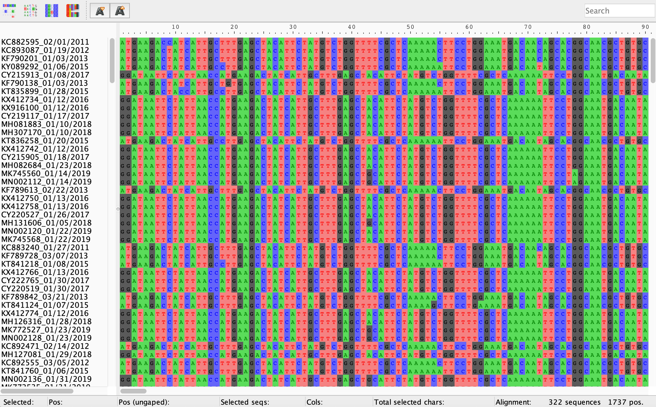
Click the Align drop down menu and then choose Realign everything. AliView will align our sequences using Muscle by default, which should only take a few minutes for a dataset of this size. All columns should now for the most part have the same nucleotide base except for columns with single nucleotide polymorphisms or insertions/deletions (i.e. indels).
Hint: In AliView, you can easily zoom in and out on an alignment by holding Command + scrolling up and down. This is an easy way to get a bird’s eye view of your alignment before making sure each site is properly aligned.
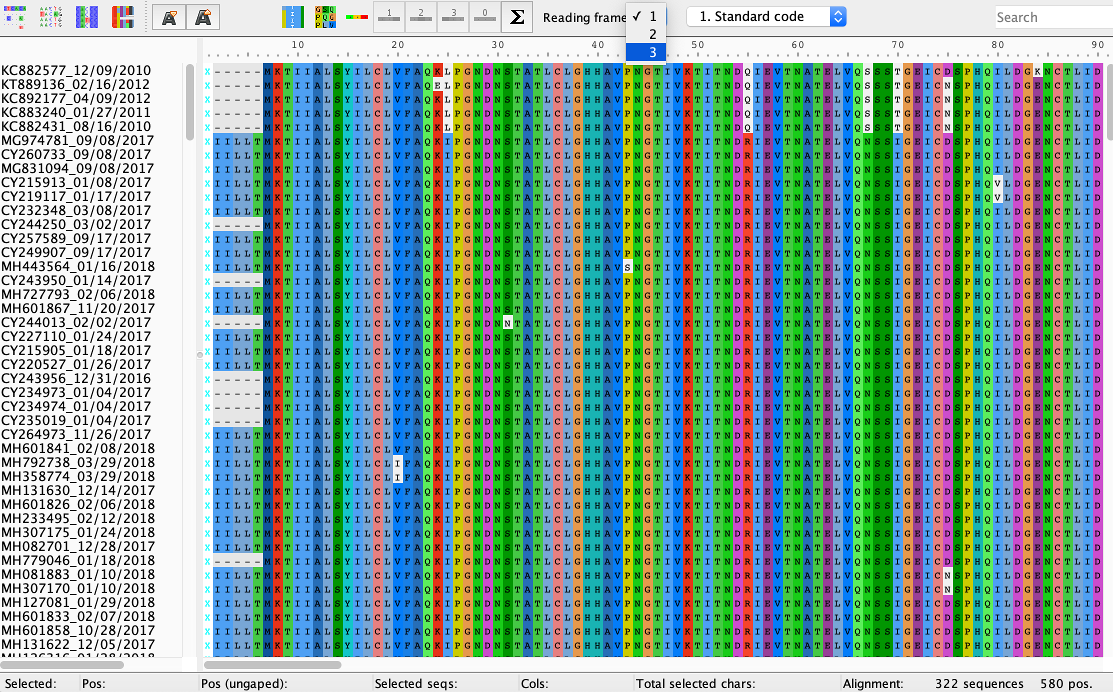
For protein coding sequences like the HA gene, it is a good idea to make sure sequences are aligned at the amino acid as well as the nucleotide level because misaligned sequences can often be easily spotted by an excess of stop codons and/or missense mutations. In Aliview, click View → Show as translation (Command + T). We won’t necessarily know where the coding region begins or which reading frame we are supposed to be in, but remember that protein coding sequences always begin with a start codon ATG encoding for methionine. You can change the reading frame from the Reading frame drop down menu at the top of the alignment window. If the sequences are correctly aligned, there should be a high degree of conservation among amino acid residues at each site and no premature stop codons. The figure below provides a hint if you cannot guess the correct reading frame.
Brain stretcher: People most often reconstruct phylogenies from nucleotide sequence data, although sometimes researchers use translated amino acid alignments. Can you think of situations where it might be preferable to reconstruct trees from amino acid instead of nucleotide sequences?
Export the nucleotide alignment as a fasta file by selecting File → Save as Fasta. You may want to name the new fasta file to denote that these are aligned sequences, like influenzaA_H3N2_NC_2010-2019_aligned.fasta.
Reconstructing a maximum likelihood phylogeny
We will learn more about how likelihood-based phylogenetic reconstruction works in week three. For now, we’ll use RAxML-NG to build our first phylogeny. Precompiled versions of RAxML-NG are available from the RAxML-NG GitHub repo. Alternatively, if you installed Anaconda, you can install RAxML-NG using conda from the command line: conda install bioconda::raxml-ng. If for some reason you cannot get RAxML installed on your own machine, you can run it remotely on the CIPRES Science Gateway.
Hint: We will not be working extensively from the command line in the class, but knowing some basics can be very helpful. I recommend this fantastic tutorial from sandbox.bio.
Brain stretcher: How would you count the number of sequences in a Fasta file from the command line without opening the file?
Hopefully one way or another you were able to get RAxML installed. You can check that RAxML is installed by running raxml-ng -v from the command line (Terminal on a Mac), which should display the version.
Hint: For Mac and Linux users you may want to access an executable program like RAxML from any file directory. You can modify your ENV PATH variable to point your OS towards the file path of your executable. For example you could add the path to RAxML-NG using:
export PATH=$PATH:/Applications/raxml-ng_v1.2.1_macos_x86_64/raxml-ng
Alternatively, sometimes I move commonly used programs directly to my /usr/local/bin directory so I can easily access it anywhere without worrying about modifying paths.
cp /Applications/raxml-ng_v1.2.1_macos_x86_64/raxml-ng /usr/local/bin
Note for Mac users: Mac OS may initially block you from opening the RAxML executable the first time you try to run the application. You can work around this by going to System Preferences → Privacy & Security → Security and then clicking Allow Anyway next to the message that says RAxML was blocked from opening.
___
Now we can build some trees! From the command line we can now run RAxML with our influenza alignment. Two important things to note before you do: 1) You will need to be in the same directory where you installed RAxML unless you added into to your ENV path or moved it to /usr/local/bin/ as shown in the Hint above. 2) If you are not working from the directory with the alignment file, you will need to provide the full path to the alignment file influenzaA_H3N2_NC_2010-2019_aligned.fasta, i.e. you will need to replace the path_to_file stand-in below:
raxml-ng --search1 --msa /path_to_file/influenzaA_H3N2_NC_2010-2019_aligned.fasta --model GTR+G
RAxML will then perform a fast heuristic (i.e. not exhaustive but good enough) search for the tree that maximizes the likelihood of our sequence data. The –model GTR+G argument tells RAxML that we want to use a General Time Reversible (GTR) model of molecular evolution but allow for gamma distributed rate heterogeneity among sites.
It should only take RAxML a few minutes to find the best ML tree, which will be output in a file called influenzaA_H3N2_NC_2010-2019_aligned.fasta.raxml.bestTree. You may want to add a .tre extension to this file name so we know this is a Newick tree file.
The –search1 argument tells RAxML to do a quick and dirty search starting from a single initial tree. But RAxML’s search algorithm is not guaranteed to find the best ML tree starting from any given starting tree. If you would like to perform a more exhaustive search starting from different starting trees (10 by default) you can just omit the –search1 argument from the command above.
If you are interested in learning more, there is a nice hands-on RAxML-NG tutorial.
Brain stretcher: Since RAxML uses a heuristic search algorithm to try to find the best ML tree, how could we compare trees across multiple searches to ensure we’re getting a good enough tree?
Viewing our tree in FigTree
Open FigTree and then load the ML phylogeny we just reconstructed using File → Open.
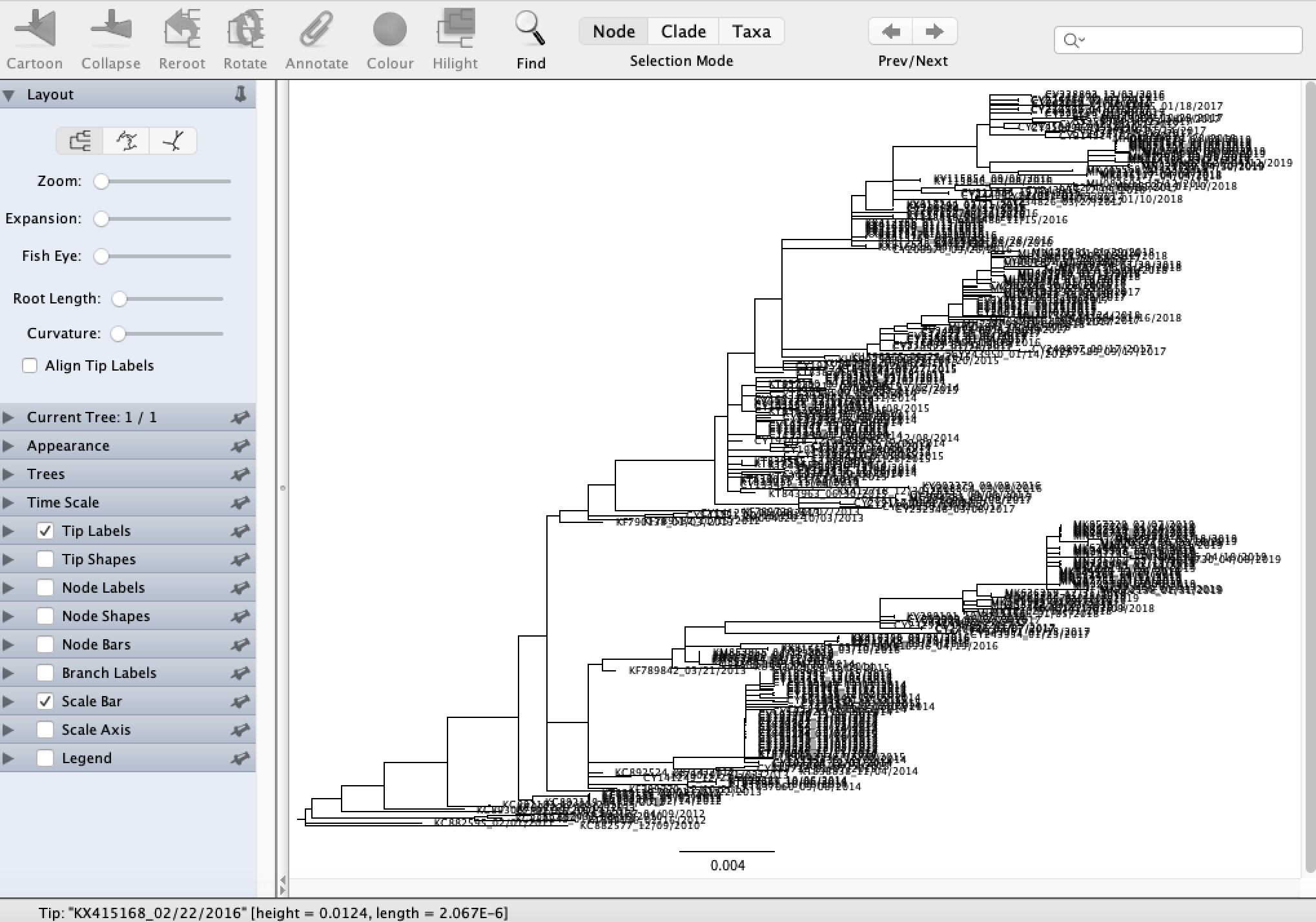
We can see right away that there is a great deal of temporal structure to the tree topology: sequences sampled in the same flu season generally tend to cluster together, which is what we expect. FigTree has a bunch of nice features for viewing phylogenies that you should take a few minutes to explore. For example, you can explore different tree layouts, change the tree appearance and annotate the nodes and branches in the tree with different metadata.
Testing the molecular clock assumption
Note that branch lengths in the tree are given in terms of substitutions, not in units of real time. In the third week we will look into Bayesian approaches for reconstructing time-calibrated phylogenies with branch lengths in units of real time. But dating phylogenies requires us to make an assumption about the molecular clock, namely that substitutions accumulate along lineages in the tree at a roughly constant rate. If this is true, two lineages sampled at the present should have accumulated roughly the same number of substitutions since they last shared a most recent common ancestor (MRCA).
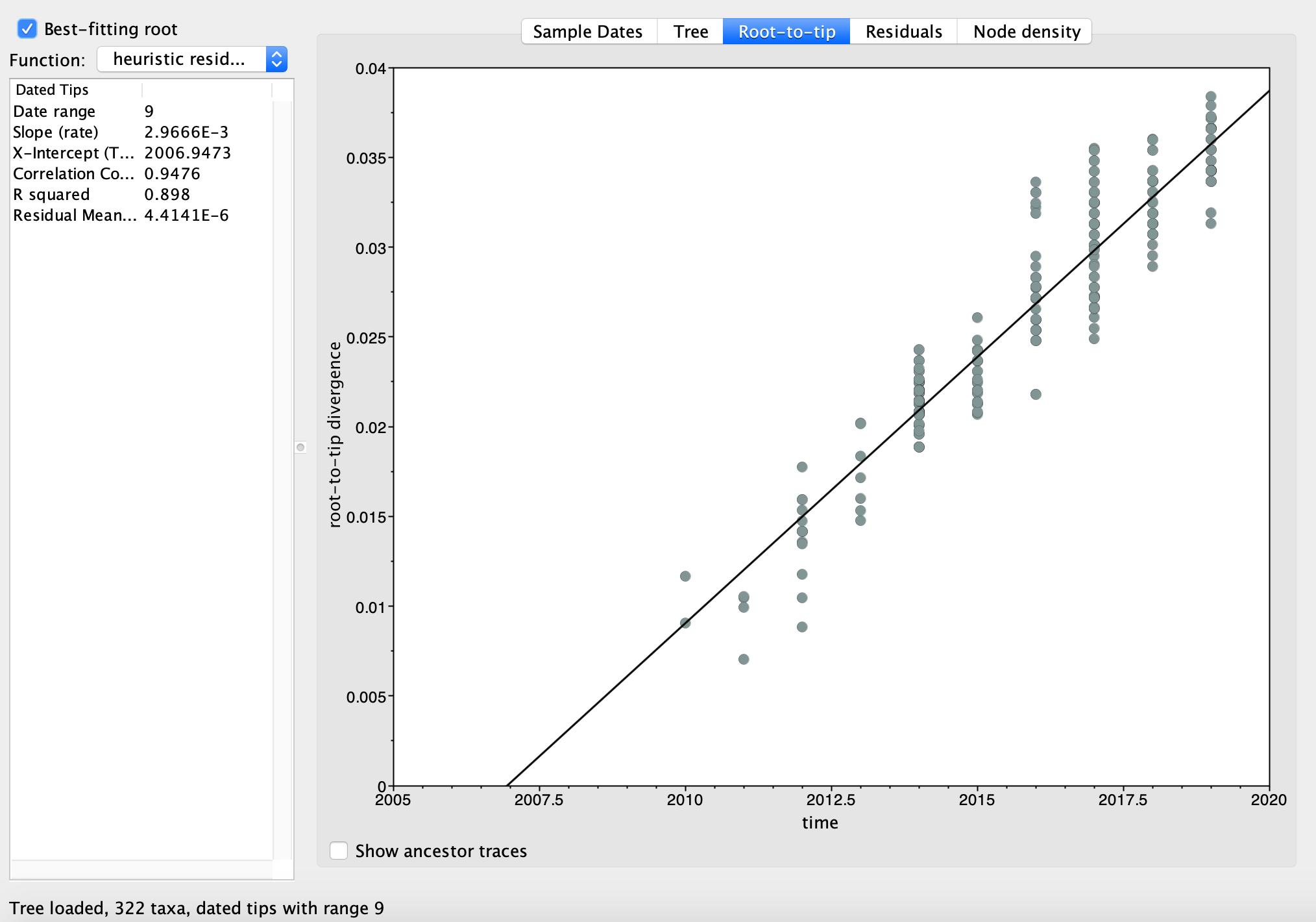
One way to test the molecular clock assumption is therefore to regress root-to-tip distances (in units of substitutions) against sample times. Since all sampled lineages share a common ancestor at the root of the tree, the number of substitutions separating each sample (tip) from the root should be proportional to the time elapsed between the root and each lineage’s sampling time. We therefore expect a roughly linear relationship between the root-to-tip distances and sampling times if the molecular clock assumption holds. Moreover, the slope of the resulting regression line will provide us with a rough estimate of the rate at which substitutions accumulate, i.e. the molecular clock rate.
TempEst provides an easy way of testing the assumption of clock-like evolution. Open TempEst and then open the influenzaA_H3N2_NC_2010-2019_aligned.fasta.raxml.bestTree ML phylogeny we reconstructed before in the pop up window that opens automatically.
Click on Parse Dates and in the pop up window that opens, select Defined just by its order and then select Last in the Order drop down menu below. You can leave Parse as number selected, then click OK. The Date column next to the name of each sequence should now be auto-populated with the correct tip dates (we will loose some info about the exact day of sampling but that’s ok). Select the Best-fitting root box at the top left of the window. Now navigate to the Root-to-tip panel. In the resulting least-squares regression plot we can see that the root-to-tip distance increases almost perfectly linearly with the sample times. Moreover, the slope of the regression line is about 3.0 X 10^-3, a very reasonable molecular clock rate for a RNA virus. The molecular clock assumption therefore seems perfectly reasonable for our flu samples, and we are all set to start reconstructing time-calibrated phylogenies using molecular clock models in BEAST 2 next week.